This page was generated from
docs/Examples/Melt_Inclusion_FeMg_Equilibrium/Ol_Melt_Inclusion_Mg_Fe_Eq_MultipleSamples.ipynb.
Interactive online version:
![]() .
.
Multisample - Fe-Mg equilibrium in ol-hosted MIs
This notebook shows how to assess Fe-Mg equilibrium between olivines and melt inclusions, and between melt inclusions and co-erupted matrix glasses to let you assess Fe-Mg diffusion and post-entrapment crystallization
In this example, we have multiple samples in the spreadsheet, so first subsample out the rows we want based on sample name. You will have to change the sample names to reflect whatever column you use for this. Else, see single sample if you only have 1 sample in your spreadsheet
You can download the spreadsheet here: https://github.com/PennyWieser/Thermobar/blob/main/docs/Examples/Melt_Inclusion_FeMg_Equilibrium/2018_MIs_Glasses.xlsx
These plots are really for matrix glass data - if its whole-rock, your Mg-Fe equilibrium could be affected by olivine addition/subtraction, and you will need to consider this
[1]:
## Install Thermobar if you haven't already (remove # and press run)

# !pip install Thermobar
[2]:
# Loading various python things
import numpy as np
import pandas as pd
import matplotlib.pyplot as plt
import Thermobar as pt
Loading a dataset
This dataset is from Wieser et al. (2021) - https://doi.org/10.1029/2020GC009364
It shows olivine-hosted melt inclusions from Fissure 8, which have undergone extensive and variable amonuts of PEC.
We load in measured melt inclusion compositions (e.g. before PEC correction), and host olivines, as well as the composition of the co-erupted matrix glass
You can download the spreadsheet here - https://github.com/PennyWieser/Thermobar/blob/main/docs/Examples/Melt_Inclusion_FeMg_Equilibrium/2018_MIs_Glasses.xlsx
Load in the matrix glasses
[3]:
# We dont have to add _Liq as its all liquids,
# just specify the _Liq in the import
MG_input=pt.import_excel('2018_MIs_Glasses.xlsx',
                         sheet_name='Matrix_Glasses', suffix="_Liq")
MG_all=MG_input['my_input'] ## All columns
MG_Liqs=MG_input['Liqs'] ## Just Liquid columns
MG_Liqs.head()
[3]:
| SiO2_Liq | TiO2_Liq | Al2O3_Liq | FeOt_Liq | MnO_Liq | MgO_Liq | CaO_Liq | Na2O_Liq | K2O_Liq | Cr2O3_Liq | P2O5_Liq | H2O_Liq | Fe3Fet_Liq | NiO_Liq | CoO_Liq | CO2_Liq | Sample_ID_Liq | |
|---|---|---|---|---|---|---|---|---|---|---|---|---|---|---|---|---|---|
| 0 | 50.6243 | 2.8773 | 13.0360 | 11.8288 | 0.1830 | 5.8471 | 10.2471 | 2.5120 | 0.5234 | 0.0 | 0.2689 | 0.0 | 0.0 | 0.0 | 0.0 | 0.0 | 0 |
| 1 | 50.0975 | 2.8840 | 12.8885 | 11.2897 | 0.1769 | 5.8521 | 9.9658 | 2.4681 | 0.5305 | 0.0 | 0.2652 | 0.0 | 0.0 | 0.0 | 0.0 | 0.0 | 1 |
| 2 | 50.1517 | 2.5827 | 13.0277 | 11.2420 | 0.2141 | 6.6763 | 10.6820 | 2.2884 | 0.4462 | 0.0 | 0.2068 | 0.0 | 0.0 | 0.0 | 0.0 | 0.0 | 2 |
| 3 | 50.2523 | 2.5686 | 13.1034 | 10.9155 | 0.1948 | 6.4934 | 10.7276 | 2.3660 | 0.4822 | 0.0 | 0.2329 | 0.0 | 0.0 | 0.0 | 0.0 | 0.0 | 3 |
| 4 | 51.1145 | 2.6104 | 13.2432 | 11.1522 | 0.1738 | 6.5764 | 10.6298 | 2.4155 | 0.4704 | 0.0 | 0.2393 | 0.0 | 0.0 | 0.0 | 0.0 | 0.0 | 4 |
Load in the melt inclusion data and the olivines
As they are in the same sheet, we have to make sure we have _Liq after the melt inclusion oxide, and _Ol after the olivine
[4]:
MIs_in=pt.import_excel('2018_MIs_Glasses.xlsx',
                         sheet_name='MIs_Ols')
MIs_Ol=MIs_in['Ols']
MIs_Liq=MIs_in['Liqs']
MIs_input=MIs_in['my_input']
Find each sample for melt inclusions
[5]:
MIs_LL4_index=MIs_input['SpecificID']=="LL4"
MIs_LL7_index=MIs_input['SpecificID']=="LL7"
MIs_LL8_index=MIs_input['SpecificID']=="LL8"
Find each sample for Glasses
[6]:
MGs_LL4_index=MG_all['SpecificID']=="LL4"
MGs_LL7_index=MG_all['SpecificID']=="LL7"
MGs_LL8_index=MG_all['SpecificID']=="LL8"
Workflow 1: Assess if the olivines are in equilibrium with the co-erupted matrix glass
1. Calculate Mg# for liquids
[7]:
Liq_Mgno_calc=pt.calculate_liq_mgno(liq_comps=MG_Liqs, Fe3Fet_Liq=0.15)

Liq_Mgno_calc.head()

# Calculate mean value to plot for each sample
Liq_Mgno_calc_mean_LL4=np.mean(Liq_Mgno_calc.loc[MGs_LL4_index])
Liq_Mgno_calc_mean_LL7=np.mean(Liq_Mgno_calc.loc[MGs_LL7_index])
Liq_Mgno_calc_mean_LL8=np.mean(Liq_Mgno_calc.loc[MGs_LL8_index])
2. Calculate Olivine Fo contents
[8]:
Ol_Fo_Calc=pt.calculate_ol_fo(ol_comps=MIs_Ol)
3. Calculate fields you want to plot on a Rhodes diagram
[9]:
Rhodes=pt.calculate_ol_rhodes_diagram_lines(Min_Mgno=0.5, Max_Mgno=0.7)
Rhodes.head()
[9]:
| Mg#_Liq | Eq_Ol_Fo_Roeder (Kd=0.3) | Eq_Ol_Fo_Roeder (Kd=0.27) | Eq_Ol_Fo_Roeder (Kd=0.33) | Eq_Ol_Fo_Matzen (Kd=0.34) | Eq_Ol_Fo_Matzen (Kd=0.328) | Eq_Ol_Fo_Matzen (Kd=0.352) | |
|---|---|---|---|---|---|---|---|
| 0 | 0.500000 | 0.769231 | 0.787402 | 0.751880 | 0.746269 | 0.753012 | 0.739645 |
| 1 | 0.502020 | 0.770662 | 0.788751 | 0.753384 | 0.747796 | 0.754512 | 0.741198 |
| 2 | 0.504040 | 0.772087 | 0.790095 | 0.754883 | 0.749317 | 0.756006 | 0.742745 |
| 3 | 0.506061 | 0.773506 | 0.791432 | 0.756375 | 0.750832 | 0.757493 | 0.744286 |
| 4 | 0.508081 | 0.774919 | 0.792763 | 0.757861 | 0.752341 | 0.758975 | 0.745822 |
4. Plot the Kd model you want, along with the olivine and glass Mg
[10]:
fig, (ax1, ax2) = plt.subplots(1, 2, figsize=(12,5))

# Plotting for Roeder and Emslie
ax1.set_title('Roeder and Emslie, 1970')
# Plotting equilibrium lines
ax1.plot(Rhodes['Mg#_Liq'], Rhodes['Eq_Ol_Fo_Roeder (Kd=0.27)'], ':k')
ax1.plot(Rhodes['Mg#_Liq'], Rhodes['Eq_Ol_Fo_Roeder (Kd=0.33)'], ':k')
ax1.plot(Rhodes['Mg#_Liq'], Rhodes['Eq_Ol_Fo_Roeder (Kd=0.3)'], '-k')

# Plotting data

ax1.plot(Ol_Fo_Calc.loc[MIs_LL4_index]*0+Liq_Mgno_calc_mean_LL4,
         Ol_Fo_Calc.loc[MIs_LL4_index], 'ok', mfc='blue')

ax1.plot(Ol_Fo_Calc.loc[MIs_LL7_index]*0+Liq_Mgno_calc_mean_LL7,
         Ol_Fo_Calc.loc[MIs_LL7_index], 'ok', mfc='orange')

ax1.plot(Ol_Fo_Calc.loc[MIs_LL8_index]*0+Liq_Mgno_calc_mean_LL8,
         Ol_Fo_Calc.loc[MIs_LL8_index], 'ok', mfc='red')

ax2.set_title('Matzen (2011)')
# Plotting equilibrium lines
ax2.plot(Rhodes['Mg#_Liq'], Rhodes['Eq_Ol_Fo_Matzen (Kd=0.328)'], ':k')
ax2.plot(Rhodes['Mg#_Liq'], Rhodes['Eq_Ol_Fo_Matzen (Kd=0.352)'], ':k')
ax2.plot(Rhodes['Mg#_Liq'], Rhodes['Eq_Ol_Fo_Matzen (Kd=0.34)'], '-k')
# Plotting data
ax2.plot(Ol_Fo_Calc.loc[MIs_LL4_index]*0+Liq_Mgno_calc_mean_LL4,
         Ol_Fo_Calc.loc[MIs_LL4_index], 'ok', mfc='blue')

ax2.plot(Ol_Fo_Calc.loc[MIs_LL7_index]*0+Liq_Mgno_calc_mean_LL7,
         Ol_Fo_Calc.loc[MIs_LL7_index], 'ok', mfc='orange')

ax2.plot(Ol_Fo_Calc.loc[MIs_LL8_index]*0+Liq_Mgno_calc_mean_LL8,
         Ol_Fo_Calc.loc[MIs_LL8_index], 'ok', mfc='red')
ax1.set_ylabel('Ol Fo content')
ax1.set_xlabel('Glass Mg#')
ax2.set_xlabel('Glass Mg#')
ax1.set_ylim([0.74, 0.9])
ax2.set_ylim([0.74, 0.9])
ax1.set_xlim([0.5, 0.6])
ax2.set_xlim([0.5, 0.6])
[10]:
(0.5, 0.6)
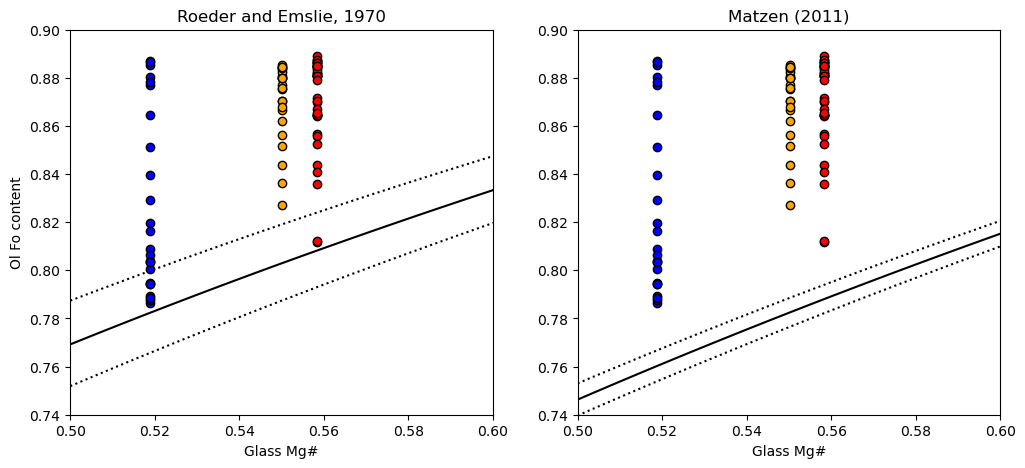
We can see that a lot of the olivines are way to primitive to be in equilibrium with the co-erupted liquid, regardless of what Kd model we use. This is the first sign that the olivines have undergone extensive post-entrapment cooling and crystallization.
Workflow 2: Assess if the olivines and their melt inclusions are in equilibrium
If post entrapment crystallization occurs, then the crystals erupt immediatly, the melt inclusion and host olivine will be out of Mg-Fe equilibirum. -However, as Danysuhevsky et al. show in a series of papers if sufficient time passes between the cooling event driving PEC and eruption, Fe-Mg will re-equilbrate, Fe will be lost from the inclusion, and the melt inclusion will re-approach equilibrium with its host olivine
1. Calculate melt inclusion Mg
[11]:
MI_Mgno_calc=pt.calculate_liq_mgno(liq_comps=MIs_Liq, Fe3Fet_Liq=0.15)
2. Plot on a rhodes diagram
[12]:
fig, (ax1, ax2) = plt.subplots(1, 2, figsize=(12,5))

# Plotting for Roeder and Emslie
ax1.set_title('Roeder and Emslie, 1970')
# Plotting equilibrium lines
ax1.plot(Rhodes['Mg#_Liq'], Rhodes['Eq_Ol_Fo_Roeder (Kd=0.27)'], ':k')
ax1.plot(Rhodes['Mg#_Liq'], Rhodes['Eq_Ol_Fo_Roeder (Kd=0.33)'], ':k')
ax1.plot(Rhodes['Mg#_Liq'], Rhodes['Eq_Ol_Fo_Roeder (Kd=0.3)'], '-k')

# Plotting data
ax1.plot(MI_Mgno_calc.loc[MIs_LL4_index], Ol_Fo_Calc.loc[MIs_LL4_index], 'ok', mfc='blue')
ax1.plot(MI_Mgno_calc.loc[MIs_LL7_index], Ol_Fo_Calc.loc[MIs_LL7_index], 'ok', mfc='orange')
ax1.plot(MI_Mgno_calc.loc[MIs_LL8_index], Ol_Fo_Calc.loc[MIs_LL8_index], 'ok', mfc='red')

ax2.set_title('Matzen (2011)')
# Plotting equilibrium lines
ax2.plot(Rhodes['Mg#_Liq'], Rhodes['Eq_Ol_Fo_Matzen (Kd=0.328)'], ':k')
ax2.plot(Rhodes['Mg#_Liq'], Rhodes['Eq_Ol_Fo_Matzen (Kd=0.352)'], ':k')
ax2.plot(Rhodes['Mg#_Liq'], Rhodes['Eq_Ol_Fo_Matzen (Kd=0.34)'], '-k')
# Plotting data
ax2.plot(MI_Mgno_calc.loc[MIs_LL4_index], Ol_Fo_Calc.loc[MIs_LL4_index], 'ok', mfc='blue')
ax2.plot(MI_Mgno_calc.loc[MIs_LL7_index], Ol_Fo_Calc.loc[MIs_LL7_index], 'ok', mfc='orange')
ax2.plot(MI_Mgno_calc.loc[MIs_LL8_index], Ol_Fo_Calc.loc[MIs_LL8_index], 'ok', mfc='red')

ax1.set_ylabel('Ol Fo content')
ax1.set_xlabel('Melt inclusion Mg#')
ax2.set_xlabel('Melt inclusion Mg#')
ax1.set_ylim([0.74, 0.92])
ax2.set_ylim([0.74, 0.92])
ax1.set_xlim([0.5, 0.7])
ax2.set_xlim([0.5, 0.7])
[12]:
(0.5, 0.7)
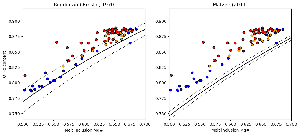
We can see using the Roeder and Emslie model, the melt inclusions are perfectly in line with the equilibrium field. Combined with the extensive olivine-matrix glass Fe-Mg disequilibrium, this shows extensive PEC, followed by diffusive re-equilibration
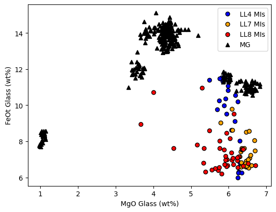
Another line of evidence comes from plotting matrix glass and melt inclusoins in MgO-FeO space, its clear MI have lost abundant Fe
[13]:
plt.plot(MIs_Liq['MgO_Liq'].loc[MIs_LL4_index], MIs_Liq['FeOt_Liq'].loc[MIs_LL4_index],
         'ok', mfc='blue', label='LL4 MIs')
plt.plot(MIs_Liq['MgO_Liq'].loc[MIs_LL7_index], MIs_Liq['FeOt_Liq'].loc[MIs_LL7_index],
         'ok', mfc='orange', label='LL7 MIs')
plt.plot(MIs_Liq['MgO_Liq'].loc[MIs_LL8_index], MIs_Liq['FeOt_Liq'].loc[MIs_LL8_index],
         'ok', mfc='red', label='LL8 MIs')
plt.plot(MG_Liqs['MgO_Liq'],MG_Liqs['FeOt_Liq'], '^k', mfc='k', label='MG')
plt.xlabel('MgO Glass (wt%)')
plt.ylabel('FeOt Glass (wt%)')
plt.legend()
[13]:
<matplotlib.legend.Legend at 0x188ca61f4c0>