This page was generated from docs/Examples/Error_propagation/Cpx_Liq_Thermobarometry_Error_prop.ipynb. Interactive online version: .

Error propagation - Cpx-Liquid.

This notebook demonstrates how to propagate errors in Cpx-Liquid thermobarometry
This builds on from the notebook showing how to consider error in a single phase (Liquid_Thermometry_error_prop.ipynb). We suggest you look at that first, as its simpler when you don’t have to worry about two separate phases
We use the experimental data of Feig et al. (2010) - DOI 10.1007/s00410-010-0493-3, and the author-stated 1 sigma errors
You can download the excel file here https://github.com/PennyWieser/Thermobar/blob/main/docs/Examples/Error_propagation/Cpx_Liq_Error_prop_Feig2010_example.xlsx

You need to install Thermobar once on your machine, if you haven’t done this yet, uncomment the line below (remove the #)

[1]:

#!pip install Thermobar

[2]:

# Import other python stuff
import numpy as np
import pandas as pd
import matplotlib.pyplot as plt
import Thermobar as pt
pd.options.display.max_columns = None
pt.__version__

[2]:

'1.0.56'

Importing data

[3]:

out=pt.import_excel('Cpx_Liq_Error_prop_Feig2010_example.xlsx', sheet_name="Sheet1")
my_input=out['my_input']
myCpxs1=out['Cpxs']
myLiquids1=out['Liqs']

[4]:

## Check input looks reasonable
display(myCpxs1.head())
display(myLiquids1.head())

	SiO2_Cpx	TiO2_Cpx	Al2O3_Cpx	FeOt_Cpx	MnO_Cpx	MgO_Cpx	CaO_Cpx	Na2O_Cpx	Cr2O3_Cpx	Sample_ID_Cpx
0	51.075956	0.325086	4.892502	5.714957	0.165700	16.897042	20.466034	0.319704	0.252186	Feig2010_1
1	51.578350	0.356860	3.600200	6.390180	0.171190	16.402000	20.388060	0.332720	0.186270	Feig2010_2
2	51.567875	0.256271	4.763807	4.229021	0.000000	16.969344	21.061352	0.316506	0.528929	Feig2010_3
3	52.083950	0.325983	3.919567	5.285317	0.168583	16.604683	20.364050	0.318067	0.377937	Feig2010_4
4	52.331846	0.406175	3.974610	6.039907	0.173175	16.297102	19.784783	0.388863	0.285975	Feig2010_5

	SiO2_Liq	TiO2_Liq	Al2O3_Liq	FeOt_Liq	MgO_Liq	CaO_Liq	Na2O_Liq	H2O_Liq	Sample_ID_Liq
0	50.973845	0.489282	19.349173	5.327336	4.511373	9.161873	4.205536	5.12	Feig2010_1
1	53.642629	0.617371	19.320971	4.884986	3.257343	6.824314	5.057043	5.18	Feig2010_2
2	49.629083	0.365787	19.103075	5.302860	6.403377	11.615943	3.275783	5.05	Feig2010_3
3	51.624314	0.443871	18.451100	6.303071	6.132229	10.365057	3.685714	2.67	Feig2010_4
4	53.980586	0.817471	17.454986	6.744429	5.149100	9.030871	4.179543	2.25	Feig2010_5

Example 1: Uncertainty in a single input parameter for Cpx-only and Cpx-Liq barometry

Here, we consider the effect of adding just 5% noise to measured Na2O contents of Cpx (a fairly typical uncertainty resulting from EPMA analyses)
Because our liquids and cpx dataframes need to be the same size to feed into the calculate_Cpx_Liq functions, we also use the add_noise_sample_1phase to generate a dataframe of Liq compositions, however, we simply state noise_percent=0 so all the rows for each liquid are identical

[5]:

# Make liquid dataframe of the right size, no noise added
Liquids_only_noNoise=pt.add_noise_sample_1phase(phase_comp=myLiquids1,
                        noise_percent=0, duplicates=1000, err_dist="normal")

All negative numbers replaced with zeros. If you wish to keep these, set positive=False

c:\users\penny\box\postdoc\mybarometers\thermobar_outer\src\Thermobar\noise_averaging.py:587: FutureWarning: Downcasting object dtype arrays on .fillna, .ffill, .bfill is deprecated and will change in a future version. Call result.infer_objects(copy=False) instead. To opt-in to the future behavior, set `pd.set_option('future.no_silent_downcasting', True)`
  mynoisedDataframe=mynoisedDataframe.fillna(0)

[6]:

# Make Cpx dataframe, with 5% random noise added to Na2O
Cpx_5Na2O=pt.add_noise_sample_1phase(phase_comp=myCpxs1, variable="Na2O",
variable_err=5, variable_err_type="Perc", duplicates=1000, err_dist="normal")

Cpx_5Na2O.head()

All negative numbers replaced with zeros. If you wish to keep these, set positive=False

c:\users\penny\box\postdoc\mybarometers\thermobar_outer\src\Thermobar\noise_averaging.py:587: FutureWarning: Downcasting object dtype arrays on .fillna, .ffill, .bfill is deprecated and will change in a future version. Call result.infer_objects(copy=False) instead. To opt-in to the future behavior, set `pd.set_option('future.no_silent_downcasting', True)`
  mynoisedDataframe=mynoisedDataframe.fillna(0)

[6]:

	SiO2_Cpx	TiO2_Cpx	Al2O3_Cpx	FeOt_Cpx	MnO_Cpx	MgO_Cpx	CaO_Cpx	Na2O_Cpx	Cr2O3_Cpx	Sample_ID_Cpx
0	51.075956	0.325086	4.892502	5.714957	0.1657	16.897042	20.466034	0.311029	0.252186	Feig2010_1
1	51.075956	0.325086	4.892502	5.714957	0.1657	16.897042	20.466034	0.321726	0.252186	Feig2010_1
2	51.075956	0.325086	4.892502	5.714957	0.1657	16.897042	20.466034	0.333426	0.252186	Feig2010_1
3	51.075956	0.325086	4.892502	5.714957	0.1657	16.897042	20.466034	0.335205	0.252186	Feig2010_1
4	51.075956	0.325086	4.892502	5.714957	0.1657	16.897042	20.466034	0.276867	0.252186	Feig2010_1

[7]:

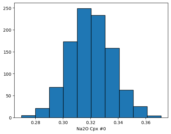
# Plot what the Na content looks like
plt.hist(Cpx_5Na2O['Na2O_Cpx'].loc[Cpx_5Na2O['Sample_ID_Cpx_Num']==0], ec='k')
plt.xlabel('Na2O Cpx #0')

[7]:

Text(0.5, 0, 'Na2O Cpx #0')

../../_images/Examples_Error_propagation_Cpx_Liq_Thermobarometry_Error_prop_10_1.png

Lets first calculate Cpx-only pressures for these synthetic noisy Cpxs

[8]:

Out_5_noise_cpx_only=pt.calculate_cpx_only_press_temp(cpx_comps=Cpx_5Na2O,
                                    equationP="P_Put2008_eq32a",
                                        equationT="T_Put2008_eq32d", eq_tests=True)
Out_5_noise_cpx_only

[8]:

	P_kbar_calc	T_K_calc	Delta_P_kbar_Iter	Delta_T_K_Iter	SiO2_Cpx	TiO2_Cpx	Al2O3_Cpx	FeOt_Cpx	MnO_Cpx	MgO_Cpx	CaO_Cpx	Na2O_Cpx	K2O_Cpx	Cr2O3_Cpx	Sample_ID_Cpx_Num	Sample_ID_Cpx	Si_Cpx_cat_6ox	Mg_Cpx_cat_6ox	Fet_Cpx_cat_6ox	Ca_Cpx_cat_6ox	Al_Cpx_cat_6ox	Na_Cpx_cat_6ox	K_Cpx_cat_6ox	Mn_Cpx_cat_6ox	Ti_Cpx_cat_6ox	Cr_Cpx_cat_6ox	oxy_renorm_factor	Al_IV_cat_6ox	Al_VI_cat_6ox	En_Simple_MgFeCa_Cpx	Fs_Simple_MgFeCa_Cpx	Wo_Simple_MgFeCa_Cpx	Cation_Sum_Cpx	Ca_CaMgFe	Lindley_Fe3_Cpx	Lindley_Fe2_Cpx	Lindley_Fe3_Cpx_prop	CrCaTs	a_cpx_En	Mgno_Cpx	Jd	Jd_from 0=Na, 1=Al	CaTs	CaTi	DiHd_1996	EnFs	DiHd_2003	Di_Cpx	FeIII_Wang21	FeII_Wang21
0	7.227835	1503.718953	0.000000e+00	0.000000e+00	51.075956	0.325086	4.892502	5.714957	0.165700	16.897042	20.466034	0.311029	0	0.252186	0	Feig2010_1	1.869449	0.921969	0.174931	0.802609	0.211050	0.022072	0.0	0.005137	0.008950	0.007297	0.0	0.130551	0.080499	0.485372	0.092093	0.422535	4.023464	0.422535	0.046927	0.128003	0.268262	0.003649	0.154244	0.840518	0.022072	0	0.058426	0.036062	0.704471	0.196214	0.704471	0.589364	0.046927	0.128003
1	7.300723	1504.165834	0.000000e+00	0.000000e+00	51.075956	0.325086	4.892502	5.714957	0.165700	16.897042	20.466034	0.321726	0	0.252186	0	Feig2010_1	1.869331	0.921911	0.174920	0.802558	0.211036	0.022830	0.0	0.005137	0.008949	0.007297	0.0	0.130669	0.080367	0.485372	0.092093	0.422535	4.023968	0.422535	0.047936	0.126983	0.274048	0.003648	0.153557	0.840518	0.022830	0	0.057537	0.036566	0.704806	0.196012	0.704806	0.589644	0.047936	0.126983
2	7.380422	1504.653239	0.000000e+00	0.000000e+00	51.075956	0.325086	4.892502	5.714957	0.165700	16.897042	20.466034	0.333426	0	0.252186	0	Feig2010_1	1.869201	0.921847	0.174908	0.802502	0.211022	0.023658	0.0	0.005136	0.008949	0.007296	0.0	0.130799	0.080223	0.485372	0.092093	0.422535	4.024520	0.422535	0.049040	0.125868	0.280377	0.003648	0.152807	0.840518	0.023658	0	0.056565	0.037117	0.705173	0.195791	0.705173	0.589951	0.049040	0.125868
3	7.392536	1504.727211	0.000000e+00	0.000000e+00	51.075956	0.325086	4.892502	5.714957	0.165700	16.897042	20.466034	0.335205	0	0.252186	0	Feig2010_1	1.869182	0.921837	0.174906	0.802494	0.211020	0.023784	0.0	0.005136	0.008949	0.007296	0.0	0.130818	0.080201	0.485372	0.092093	0.422535	4.024604	0.422535	0.049208	0.125698	0.281339	0.003648	0.152692	0.840518	0.023784	0	0.056417	0.037201	0.705228	0.195757	0.705228	0.589997	0.049208	0.125698
4	6.994893	1502.283678	0.000000e+00	0.000000e+00	51.075956	0.325086	4.892502	5.714957	0.165700	16.897042	20.466034	0.276867	0	0.252186	0	Feig2010_1	1.869827	0.922155	0.174966	0.802771	0.211092	0.019652	0.0	0.005138	0.008952	0.007299	0.0	0.130173	0.080919	0.485372	0.092093	0.422535	4.021852	0.422535	0.043704	0.131262	0.249784	0.003649	0.156442	0.840518	0.019652	0	0.061267	0.034453	0.703401	0.196860	0.703401	0.588469	0.043704	0.131262
...	...	...	...	...	...	...	...	...	...	...	...	...	...	...	...	...	...	...	...	...	...	...	...	...	...	...	...	...	...	...	...	...	...	...	...	...	...	...	...	...	...	...	...	...	...	...	...	...	...	...
6995	7.249241	1510.684274	4.547474e-13	3.865352e-12	52.498000	0.299767	3.517867	5.903067	0.178867	17.869733	19.342233	0.331537	0	0.377700	6	Feig2010_7	1.910322	0.969372	0.179638	0.754125	0.150869	0.023391	0.0	0.005513	0.008205	0.010866	0.0	0.089678	0.061191	0.509355	0.094390	0.396254	4.012301	0.396254	0.024602	0.155036	0.136951	0.005433	0.201890	0.843654	0.023391	0	0.037800	0.025939	0.684953	0.232028	0.684953	0.575108	0.024602	0.155036
6996	7.075519	1509.490172	4.547474e-13	3.865352e-12	52.498000	0.299767	3.517867	5.903067	0.178867	17.869733	19.342233	0.306733	0	0.377700	6	Feig2010_7	1.910601	0.969513	0.179664	0.754235	0.150891	0.021644	0.0	0.005514	0.008206	0.010867	0.0	0.089399	0.061492	0.509355	0.094390	0.396254	4.011136	0.396254	0.022271	0.157392	0.123962	0.005434	0.203569	0.843654	0.021644	0	0.039848	0.024776	0.684178	0.232500	0.684178	0.574457	0.022271	0.157392
6997	7.179513	1510.205365	4.547474e-13	3.865352e-12	52.498000	0.299767	3.517867	5.903067	0.178867	17.869733	19.342233	0.321582	0	0.377700	6	Feig2010_7	1.910434	0.969429	0.179648	0.754170	0.150878	0.022690	0.0	0.005513	0.008205	0.010866	0.0	0.089566	0.061312	0.509355	0.094390	0.396254	4.011833	0.396254	0.023667	0.155982	0.131738	0.005433	0.202563	0.843654	0.022690	0	0.038622	0.025472	0.684642	0.232217	0.684642	0.574846	0.023667	0.155982
6998	7.383643	1511.605930	0.000000e+00	0.000000e+00	52.498000	0.299767	3.517867	5.903067	0.178867	17.869733	19.342233	0.350721	0	0.377700	6	Feig2010_7	1.910107	0.969263	0.179617	0.754040	0.150852	0.024741	0.0	0.005512	0.008204	0.010865	0.0	0.089893	0.060959	0.509355	0.094390	0.396254	4.013202	0.396254	0.026403	0.153214	0.146997	0.005432	0.200594	0.843654	0.024741	0	0.036217	0.026838	0.685553	0.231664	0.685553	0.575611	0.026403	0.153214
6999	7.086674	1509.566941	4.547474e-13	3.865352e-12	52.498000	0.299767	3.517867	5.903067	0.178867	17.869733	19.342233	0.308326	0	0.377700	6	Feig2010_7	1.910583	0.969504	0.179662	0.754228	0.150890	0.021756	0.0	0.005514	0.008206	0.010867	0.0	0.089417	0.061473	0.509355	0.094390	0.396254	4.011211	0.396254	0.022421	0.157241	0.124796	0.005434	0.203461	0.843654	0.021756	0	0.039716	0.024850	0.684228	0.232469	0.684228	0.574498	0.022421	0.157241

7000 rows × 50 columns

Lets plot the distribution of pressures for each Cpx

[9]:

fig, ((ax1, ax2), (ax3, ax4), (ax5, ax6)) = plt.subplots(3, 2, figsize=(10, 10))

ax1.hist(Out_5_noise_cpx_only.loc[Out_5_noise_cpx_only['Sample_ID_Cpx_Num']==0, "P_kbar_calc"], bins=50, ec='k', density = True)
ax1.annotate("Cpx 1", xy=(0.02, 0.9), xycoords="axes fraction", fontsize=9)
ax2.hist(Out_5_noise_cpx_only.loc[Out_5_noise_cpx_only['Sample_ID_Cpx_Num']==1, "P_kbar_calc"], bins=50, ec='k', density = True)
ax2.annotate("Cpx 2", xy=(0.02, 0.9), xycoords="axes fraction", fontsize=9)
ax3.hist(Out_5_noise_cpx_only.loc[Out_5_noise_cpx_only['Sample_ID_Cpx_Num']==2, "P_kbar_calc"], bins=50, ec='k', density = True)
ax3.annotate("Cpx 3", xy=(0.02, 0.9), xycoords="axes fraction", fontsize=9)
ax4.hist(Out_5_noise_cpx_only.loc[Out_5_noise_cpx_only['Sample_ID_Cpx_Num']==3, "P_kbar_calc"], bins=50, ec='k', density = True)
ax4.annotate("Cpx 4", xy=(0.02, 0.9), xycoords="axes fraction", fontsize=9)
ax5.hist(Out_5_noise_cpx_only.loc[Out_5_noise_cpx_only['Sample_ID_Cpx_Num']==4, "P_kbar_calc"], bins=50, ec='k', density = True)
ax5.annotate("Cpx 5", xy=(0.02, 0.9), xycoords="axes fraction", fontsize=9)
ax6.hist(Out_5_noise_cpx_only.loc[Out_5_noise_cpx_only['Sample_ID_Cpx_Num']==5, "P_kbar_calc"], bins=50, ec='k', density = True)
ax6.annotate("Cpx 6", xy=(0.02, 0.9), xycoords="axes fraction", fontsize=9)

ax1.set_xlabel('Pressure (kbar)')
ax2.set_xlabel('Pressure (kbar)')
ax4.set_xlabel('Pressure (kbar)')
ax3.set_xlabel('Pressure (kbar)')
ax6.set_xlabel('Pressure (kbar)')
ax5.set_xlabel('Pressure (kbar)')
ax1.set_ylabel('Probability Density')
ax3.set_ylabel('Probability Density')
ax5.set_ylabel('Probability Density')
plt.rcParams['figure.dpi']= 300

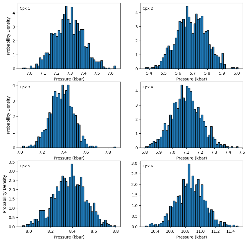
../../_images/Examples_Error_propagation_Cpx_Liq_Thermobarometry_Error_prop_14_0.png

We can also calculate statistics…

The first input is the thing you want to average (e.g. the calculated temperature in this instance), the second input is the thing you want to do the averaging based on (e.g. here average all rows with the same value of “Sample_ID_Liq_Num”

[10]:

Stats_T_K_cpx_only_5=pt.av_noise_samples_series(calc=Out_5_noise_cpx_only['T_K_calc'],
                                     sampleID=Out_5_noise_cpx_only['Sample_ID_Cpx_Num'])
Stats_T_K_cpx_only_5

[10]:

	Sample	# averaged	Mean_calc	Median_calc	St_dev_calc	St_dev_calc_from_percentiles	Max_calc	Min_calc
0	0	1000	1504.099387	1504.106545	0.653346	0.643793	1506.036798	1501.817177
1	1	1000	1482.805655	1482.805494	0.612961	0.607702	1484.679194	1480.991890
2	2	1000	1513.507632	1513.516422	0.608035	0.589460	1515.200581	1511.724035
3	3	1000	1505.893796	1505.895598	0.714193	0.717922	1508.272662	1503.450884
4	4	1000	1512.128554	1512.158212	0.932246	0.908063	1515.192833	1508.637126
5	5	1000	1542.924977	1542.939859	1.255168	1.240650	1547.274732	1538.791547
6	6	1000	1510.239702	1510.246361	0.809433	0.827093	1512.609976	1508.068596

[11]:

Stats_P_kbar_cpx_only_5=pt.av_noise_samples_series(calc=Out_5_noise_cpx_only['P_kbar_calc'],
                                     sampleID=Out_5_noise_cpx_only['Sample_ID_Cpx_Num'])
Stats_P_kbar_cpx_only_5

[11]:

	Sample	# averaged	Mean_calc	Median_calc	St_dev_calc	St_dev_calc_from_percentiles	Max_calc	Min_calc
0	0	1000	7.290062	7.291043	0.106654	0.105089	7.607838	6.919548
1	1	1000	5.687446	5.687179	0.104599	0.103738	6.009297	5.379663
2	2	1000	7.377773	7.379029	0.106852	0.103605	7.677363	7.066404
3	3	1000	7.095341	7.095423	0.115172	0.115768	7.481146	6.703539
4	4	1000	8.374863	8.379182	0.142349	0.138658	8.844933	7.844358
5	5	1000	10.870135	10.872028	0.191941	0.189681	11.539521	10.241823
6	6	1000	7.184615	7.185479	0.117798	0.120363	7.530379	6.869288

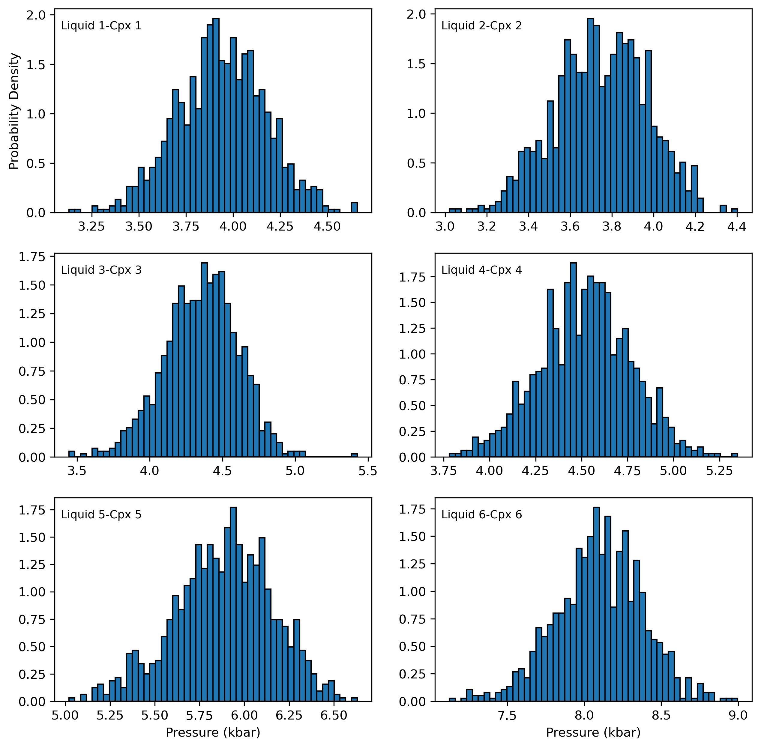
Lets do the same but for Cpx-Liq now. Remember, only Cpx has noise added

here, T=equation 33 from Putirka 2008, P=Equation 31 from Putirka 2008

[12]:

Out_5_noise_cpx_liq=pt.calculate_cpx_liq_press_temp(liq_comps=Liquids_only_noNoise, cpx_comps=Cpx_5Na2O,
                                    equationP="P_Put2008_eq31", equationT="T_Put2008_eq33", eq_tests=True)

Using Fe3FeT from input file to calculate Kd Fe-Mg

Each histogram shows the pressure distribution from a single Cpx-Liquid pair resulting from adding 5% error to just Na in Cpx.

Here we use the loc function to find all the rows where Cpx_Num==0, e.g. this is the first liquid in your excel spreadsheet.
If you wanted the 6th liquid instead, change ==0 to ==5 (as python starts its numbering from 0)

[13]:

fig, ((ax1, ax2), (ax3, ax4), (ax5, ax6)) = plt.subplots(3, 2, figsize=(10, 10))

ax1.hist(Out_5_noise_cpx_liq.loc[Out_5_noise_cpx_liq['Sample_ID_Cpx_Num']==0, "P_kbar_calc"], bins=50, ec='k', density = True)
ax1.annotate("Liquid 1-Cpx 1", xy=(0.02, 0.9), xycoords="axes fraction", fontsize=9)
ax2.hist(Out_5_noise_cpx_liq.loc[Out_5_noise_cpx_liq['Sample_ID_Cpx_Num']==1, "P_kbar_calc"], bins=50, ec='k', density = True)
ax2.annotate("Liquid 2-Cpx 2", xy=(0.02, 0.9), xycoords="axes fraction", fontsize=9)
ax3.hist(Out_5_noise_cpx_liq.loc[Out_5_noise_cpx_liq['Sample_ID_Cpx_Num']==2, "P_kbar_calc"], bins=50, ec='k', density = True)
ax3.annotate("Liquid 3-Cpx 3", xy=(0.02, 0.9), xycoords="axes fraction", fontsize=9)
ax4.hist(Out_5_noise_cpx_liq.loc[Out_5_noise_cpx_liq['Sample_ID_Cpx_Num']==3, "P_kbar_calc"], bins=50, ec='k', density = True)
ax4.annotate("Liquid 4-Cpx 4", xy=(0.02, 0.9), xycoords="axes fraction", fontsize=9)
ax5.hist(Out_5_noise_cpx_liq.loc[Out_5_noise_cpx_liq['Sample_ID_Cpx_Num']==4, "P_kbar_calc"], bins=50, ec='k', density = True)
ax5.annotate("Liquid 5-Cpx 5", xy=(0.02, 0.9), xycoords="axes fraction", fontsize=9)
ax6.hist(Out_5_noise_cpx_liq.loc[Out_5_noise_cpx_liq['Sample_ID_Cpx_Num']==5, "P_kbar_calc"], bins=50, ec='k', density = True)
ax6.annotate("Liquid 6-Cpx 6", xy=(0.02, 0.9), xycoords="axes fraction", fontsize=9)

ax6.set_xlabel('Pressure (kbar)')
ax5.set_xlabel('Pressure (kbar)')
ax1.set_ylabel('Probability Density')
plt.rcParams['figure.dpi']= 300

../../_images/Examples_Error_propagation_Cpx_Liq_Thermobarometry_Error_prop_21_0.png

Calculate Statistics

[14]:

Stats_T_K_Cpx_Liq_5Na=pt.av_noise_samples_series(calc=Out_5_noise_cpx_liq['T_K_calc'],
                                     sampleID=Out_5_noise_cpx_liq['Sample_ID_Liq_Num'])
Stats_T_K_Cpx_Liq_5Na

[14]:

	Sample	# averaged	Mean_calc	Median_calc	St_dev_calc	St_dev_calc_from_percentiles	Max_calc	Min_calc
0	0	1000	1345.001843	1345.074924	2.322891	2.285465	1351.535199	1336.307678
1	1	1000	1300.431514	1300.475418	2.152045	2.122137	1306.644758	1293.712842
2	2	1000	1384.054235	1384.141741	2.580826	2.493901	1390.904971	1376.089322
3	3	1000	1397.574478	1397.643419	2.808821	2.818199	1406.342411	1387.249763
4	4	1000	1402.178783	1402.325239	2.728007	2.649773	1410.581059	1391.113363
5	5	1000	1472.955303	1473.057123	3.093181	3.056511	1483.029175	1462.048994
6	6	1000	1480.785662	1480.886904	3.308911	3.378568	1489.942710	1471.427646

[15]:

Stats_P_kbar_Cpx_Liq_5Na=pt.av_noise_samples_series(calc=Out_5_noise_cpx_liq['P_kbar_calc'],
                                     sampleID=Out_5_noise_cpx_liq['Sample_ID_Liq_Num'])
Stats_P_kbar_Cpx_Liq_5Na

[15]:

	Sample	# averaged	Mean_calc	Median_calc	St_dev_calc	St_dev_calc_from_percentiles	Max_calc	Min_calc
0	0	1000	3.940364	3.947781	0.235488	0.231689	4.602671	3.058791
1	1	1000	3.744530	3.749123	0.226668	0.223522	4.399247	3.037068
2	2	1000	4.354753	4.363423	0.255596	0.246982	5.033238	3.565857
3	3	1000	4.510919	4.517674	0.274360	0.275267	5.367232	3.502071
4	4	1000	5.885295	5.899599	0.266556	0.258905	6.706414	4.804011
5	5	1000	8.099009	8.108539	0.290661	0.287207	9.046109	7.074440
6	6	1000	6.218368	6.227703	0.301218	0.307547	7.051151	5.365666

Example 2 - published absolute 1 sigma values for all oxides

Here, we use the published 1 sigma values for each oxide in both the glass and cpx reported by Feig et al. 2010
We make a noisy dataframe of the same length for liquids and cpxs, then combine them into the function for iterating P and T

First, load in the published 1 sigma values

[16]:

out_err=pt.import_excel_errors('Cpx_Liq_Error_prop_Feig2010_example.xlsx', sheet_name="Sheet1")
myLiquids1_err=out_err['Liqs_Err']
myCpxs1_err=out_err['Cpxs_Err']
myinput_Out=out_err['my_input_Err']

## Check input looks reasonable
display(myCpxs1_err.head())
display(myLiquids1_err.head())

	SiO2_Cpx_Err	TiO2_Cpx_Err	Al2O3_Cpx_Err	FeOt_Cpx_Err	MnO_Cpx_Err	MgO_Cpx_Err	CaO_Cpx_Err	Na2O_Cpx_Err	Cr2O3_Cpx_Err	Sample_ID_Cpx_Err
0	0.400044	0.032172	0.510460	0.357680	0.023249	0.538039	0.645164	0.049138	0.034646	0
1	0.628064	0.067227	0.622601	0.657476	0.050037	0.732816	1.050758	0.060948	0.062095	1
2	0.585596	0.032846	0.918768	0.506392	0.000000	0.562266	0.794310	0.107095	0.210114	2
3	0.165277	0.032709	0.240924	0.207266	0.051434	0.182666	0.355487	0.048979	0.058814	3
4	0.106509	0.040535	0.479962	0.428886	0.026673	0.431550	0.486264	0.056668	0.051372	4

	SiO2_Liq_Err	TiO2_Liq_Err	Al2O3_Liq_Err	FeOt_Liq_Err	MgO_Liq_Err	CaO_Liq_Err	Na2O_Liq_Err	H2O_Liq_Err	Sample_ID_Liq_Err
0	0.326030	0.042448	0.221884	0.432684	0.207011	0.268045	0.213647	0.2560	0
1	0.328698	0.025182	0.242675	0.214755	0.163292	0.171717	0.085388	0.2590	1
2	0.476011	0.027083	0.235814	0.301696	0.174436	0.206030	0.229583	0.2525	2
3	0.442894	0.047517	0.234808	0.219780	0.171799	0.274484	0.259757	0.1335	3
4	0.445356	0.043963	0.316155	0.389311	0.134659	0.209045	0.453723	0.1125	4

[17]:

# Make noise based on reported absolute 1 sigma errors from Feig et al (2010) for liquids
Liquids_st_noise=pt.add_noise_sample_1phase(phase_comp=myLiquids1, phase_err=myLiquids1_err,
                                             phase_err_type="Abs", duplicates=1000, err_dist="normal")

# Make noise based on reported absolute 1 sigma errors from Feig et al (2010) for Cpx
Cpxs_st_noise=pt.add_noise_sample_1phase(phase_comp=myCpxs1, phase_err=myCpxs1_err,
                                             phase_err_type="Abs", duplicates=1000, err_dist="normal")

All negative numbers replaced with zeros. If you wish to keep these, set positive=False
All negative numbers replaced with zeros. If you wish to keep these, set positive=False

[18]:

Out_st_noise=pt.calculate_cpx_liq_press_temp(liq_comps=Liquids_st_noise, cpx_comps=Cpxs_st_noise,
                                    equationP="P_Put2008_eq31",
                                    equationT="T_Put2008_eq33", eq_tests=True)
Out_st_noise['Sample_ID_Liq']=Liquids_st_noise['Sample_ID_Liq']

Using Fe3FeT from input file to calculate Kd Fe-Mg

[28]:

Out_st_noise.to_clipboard(excel=True)

[19]:

Stats_T_K_CpxLiqPubErr=pt.av_noise_samples_series(Out_st_noise['T_K_calc'], Liquids_st_noise['Sample_ID_Liq_Num'])
Stats_T_K_CpxLiqPubErr

[19]:

	Sample	# averaged	Mean_calc	Median_calc	St_dev_calc	St_dev_calc_from_percentiles	Max_calc	Min_calc
0	0.0	1000	1344.435383	1344.747707	11.229930	11.100909	1384.369104	1305.371695
1	1.0	1000	1298.013441	1299.504331	15.224302	NaN	1333.548541	1144.818839
2	2.0	1000	1381.064779	1383.753484	22.367388	NaN	1439.443767	1243.532659
3	3.0	1000	1397.042819	1397.657500	10.229309	10.033562	1431.453739	1355.934290
4	4.0	1000	1402.659713	1402.568883	10.710628	10.749283	1434.533288	1366.126111
5	5.0	1000	1473.216133	1473.096755	6.665914	6.581669	1495.696752	1453.824701
6	6.0	1000	1480.593377	1480.545522	8.976428	8.947284	1507.579100	1451.665504

[20]:

Stats_P_kbar_CpxLiqPubErr=pt.av_noise_samples_series(Out_st_noise['P_kbar_calc'], Liquids_st_noise['Sample_ID_Liq_Num'])
Stats_P_kbar_CpxLiqPubErr

[20]:

	Sample	# averaged	Mean_calc	Median_calc	St_dev_calc	St_dev_calc_from_percentiles	Max_calc	Min_calc
0	0.0	1000	3.909919	3.975865	0.819652	0.764174	6.076017	-0.016296
1	1.0	1000	3.541146	3.685400	1.396781	NaN	6.289129	-14.006508
2	2.0	1000	4.107311	4.386876	2.048212	NaN	8.415879	-10.837316
3	3.0	1000	4.463497	4.504807	0.847377	0.822174	6.545390	0.705959
4	4.0	1000	5.936478	6.000116	0.914977	0.881352	8.594677	2.659241
5	5.0	1000	8.119535	8.104446	0.449972	0.453753	9.422930	6.671740
6	6.0	1000	6.210725	6.219701	0.535385	0.520371	7.792477	4.315193

Recreate plot shown in manuscript for just 2 cpx-liq pairs from experiments

Here, on the LHS we plot cpx-liq pairs from the first row of the spreadsheet (ID=0)
On the RHS, we plot the pairs from row 4 (ID=3)

[21]:

fig, ((ax1, ax2)) = plt.subplots(1, 2, figsize=(12, 4))

ax1.hist(Out_st_noise.loc[Out_st_noise['Sample_ID_Liq_Num']==0, "P_kbar_calc"], bins=50, ec='k', density = True)
ax1.annotate("Liquid 1-Cpx 1", xy=(0.02, 0.95), xycoords="axes fraction", fontsize=9)
ax2.hist(Out_st_noise.loc[Out_st_noise['Sample_ID_Liq_Num']==3, "P_kbar_calc"], bins=50, ec='k', density = True)
ax2.annotate("Liquid 3-Cpx 3", xy=(0.02, 0.95), xycoords="axes fraction", fontsize=9)

#ax2.set_xlim([0, 6])
ax1.set_xlabel('Pressure (kbar)')
ax2.set_xlabel('Pressure (kbar)')
ax1.set_ylabel('Probability Density')
ax2.set_ylabel('Probability Density')
fig.savefig('Manuscript_2CpxNoises.png', dpi=300, transparent=True)

../../_images/Examples_Error_propagation_Cpx_Liq_Thermobarometry_Error_prop_34_0.png

Plot for 6 separate cpx-liq pairs

can average by _Cpx or _Liq, doesnt matter, as will match

[22]:

fig, ((ax1, ax2), (ax3, ax4), (ax5, ax6)) = plt.subplots(3, 2, figsize=(10, 10))

ax1.hist(Out_st_noise.loc[Out_st_noise['Sample_ID_Cpx_Num']==0, "P_kbar_calc"], bins=50, ec='k', density = True)
ax1.annotate("Liquid 1-Cpx 1", xy=(0.02, 0.9), xycoords="axes fraction", fontsize=9)


ax2.hist(Out_st_noise.loc[Out_st_noise['Sample_ID_Cpx_Num']==1, "P_kbar_calc"], bins=50, ec='k', density = True)
ax2.annotate("Liquid 2-Cpx 2", xy=(0.02, 0.9), xycoords="axes fraction", fontsize=9)

ax3.hist(Out_st_noise.loc[Out_st_noise['Sample_ID_Cpx_Num']==2, "P_kbar_calc"], bins=50, ec='k', density = True)
ax3.annotate("Liquid 3-Cpx 3", xy=(0.02, 0.9), xycoords="axes fraction", fontsize=9)

ax4.hist(Out_st_noise.loc[Out_st_noise['Sample_ID_Cpx_Num']==3, "P_kbar_calc"], bins=50, ec='k', density = True)
ax4.annotate("Liquid 4-Cpx 4", xy=(0.02, 0.9), xycoords="axes fraction", fontsize=9)

ax5.hist(Out_st_noise.loc[Out_st_noise['Sample_ID_Cpx_Num']==4, "P_kbar_calc"], bins=50, ec='k', density = True)
ax5.annotate("Liquid 5-Cpx 5", xy=(0.02, 0.9), xycoords="axes fraction", fontsize=9)

ax6.hist(Out_st_noise.loc[Out_st_noise['Sample_ID_Cpx_Num']==5, "P_kbar_calc"], bins=50, ec='k', density = True)
ax6.annotate("Liquid 6-Cpx 6", xy=(0.02, 0.9), xycoords="axes fraction", fontsize=9)

ax2.set_xlim([0, 6])
ax6.set_xlabel('Pressure (kbar)')
ax5.set_xlabel('Pressure (kbar)')
ax1.set_ylabel('Probability Density')
ax3.set_ylabel('Probability Density')
ax5.set_ylabel('Probability Density')

[22]:

Text(0, 0.5, 'Probability Density')

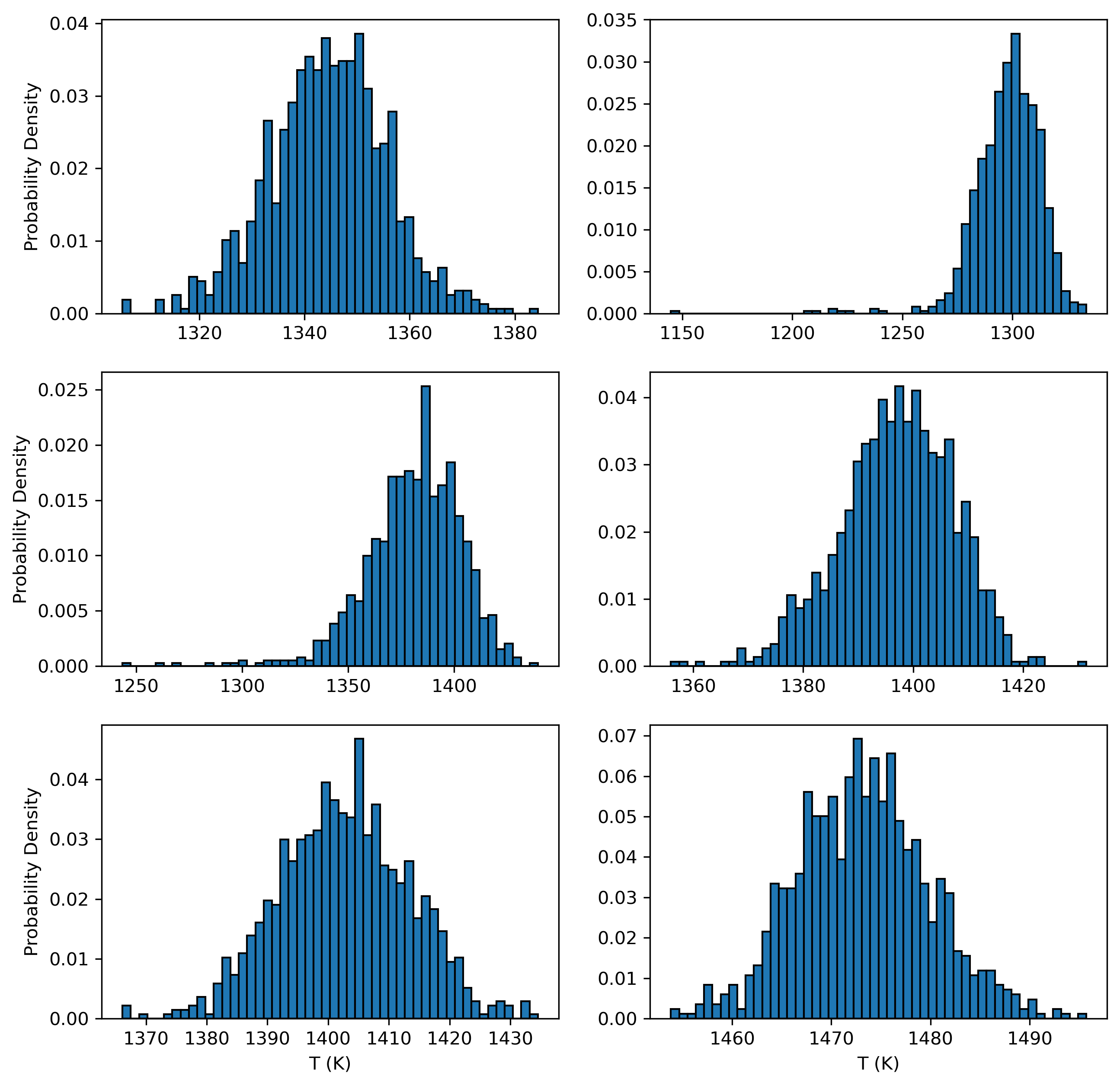
../../_images/Examples_Error_propagation_Cpx_Liq_Thermobarometry_Error_prop_36_1.png

Temperature distributions for first 6 pairs

[23]:

fig, ((ax1, ax2), (ax3, ax4), (ax5, ax6)) = plt.subplots(3, 2, figsize=(10, 10))

ax1.hist(Out_st_noise.loc[Out_st_noise['Sample_ID_Cpx_Num']==0, "T_K_calc"], bins=50, ec='k', density = True)
ax2.hist(Out_st_noise.loc[Out_st_noise['Sample_ID_Cpx_Num']==1, "T_K_calc"], bins=50, ec='k', density = True)
ax3.hist(Out_st_noise.loc[Out_st_noise['Sample_ID_Cpx_Num']==2, "T_K_calc"], bins=50, ec='k', density = True)
ax4.hist(Out_st_noise.loc[Out_st_noise['Sample_ID_Cpx_Num']==3, "T_K_calc"], bins=50, ec='k', density = True)
ax5.hist(Out_st_noise.loc[Out_st_noise['Sample_ID_Cpx_Num']==4, "T_K_calc"], bins=50, ec='k', density = True)
ax6.hist(Out_st_noise.loc[Out_st_noise['Sample_ID_Cpx_Num']==5, "T_K_calc"], bins=50, ec='k', density = True)
ax6.set_xlabel('T (K)')
ax5.set_xlabel('T (K)')
ax1.set_ylabel('Probability Density')
ax3.set_ylabel('Probability Density')
ax5.set_ylabel('Probability Density')

[23]:

Text(0, 0.5, 'Probability Density')

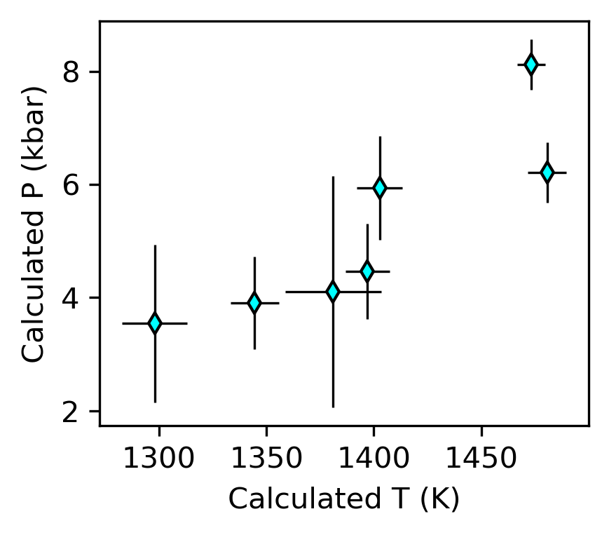
../../_images/Examples_Error_propagation_Cpx_Liq_Thermobarometry_Error_prop_38_1.png

Plots with conventional errorbars for each Cpx-Liq pair

Note, although this is typically how thermobarometric data is displayed, it isnt very realistic, our error propagation shows that error ellipses would be better - see the example below

[24]:

fig, (ax1) = plt.subplots(1, 1, figsize=(3, 2.5))

ax1.errorbar(Stats_T_K_CpxLiqPubErr['Mean_calc'],
             Stats_P_kbar_CpxLiqPubErr['Mean_calc'],
             xerr=Stats_T_K_CpxLiqPubErr['St_dev_calc'],
             yerr=Stats_P_kbar_CpxLiqPubErr['St_dev_calc'],
             fmt='d', ecolor='k', elinewidth=0.8, mfc='cyan', ms=5, mec='k')
ax1.set_ylabel('Calculated P (kbar)')
ax1.set_xlabel('Calculated T (K)')

[24]:

Text(0.5, 0, 'Calculated T (K)')

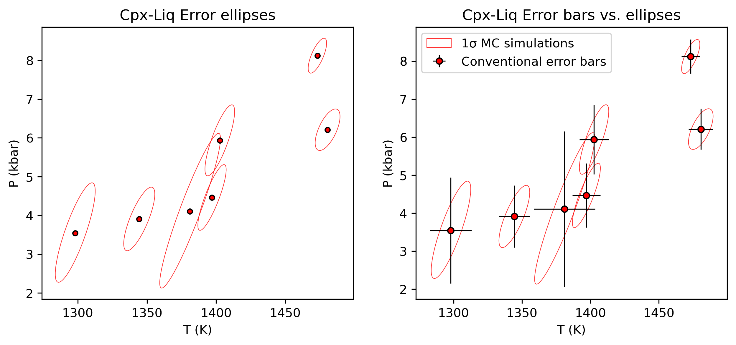
../../_images/Examples_Error_propagation_Cpx_Liq_Thermobarometry_Error_prop_40_1.png

Error ellipses instead

[25]:

Out_st_noise.columns[0:100]

[25]:

Index(['P_kbar_calc', 'T_K_calc', 'Eq Tests Neave2017?', 'Delta_P_kbar_Iter',
       'Delta_T_K_Iter', 'Delta_Kd_Put2008', 'Delta_Kd_Mas2013',
       'Delta_EnFs_Mollo13', 'Delta_EnFs_Put1999', 'Delta_CaTs_Put1999',
       'Delta_DiHd_Mollo13', 'Delta_DiHd_Put1999', 'Delta_CrCaTs_Put1999',
       'Delta_CaTi_Put1999', 'SiO2_Liq', 'TiO2_Liq', 'Al2O3_Liq', 'FeOt_Liq',
       'MnO_Liq', 'MgO_Liq', 'CaO_Liq', 'Na2O_Liq', 'K2O_Liq', 'Cr2O3_Liq',
       'P2O5_Liq', 'H2O_Liq', 'Fe3Fet_Liq', 'NiO_Liq', 'CoO_Liq', 'CO2_Liq',
       'Sample_ID_Liq_Num', 'SiO2_Liq_mol_frac', 'MgO_Liq_mol_frac',
       'MnO_Liq_mol_frac', 'FeOt_Liq_mol_frac', 'CaO_Liq_mol_frac',
       'Al2O3_Liq_mol_frac', 'Na2O_Liq_mol_frac', 'K2O_Liq_mol_frac',
       'TiO2_Liq_mol_frac', 'P2O5_Liq_mol_frac', 'Cr2O3_Liq_mol_frac',
       'Si_Liq_cat_frac', 'Mg_Liq_cat_frac', 'Mn_Liq_cat_frac',
       'Fet_Liq_cat_frac', 'Ca_Liq_cat_frac', 'Al_Liq_cat_frac',
       'Na_Liq_cat_frac', 'K_Liq_cat_frac', 'Ti_Liq_cat_frac',
       'P_Liq_cat_frac', 'Cr_Liq_cat_frac', 'Mg_Number_Liq_NoFe3',
       'Mg_Number_Liq_Fe3', 'SiO2_Cpx', 'TiO2_Cpx', 'Al2O3_Cpx', 'FeOt_Cpx',
       'MnO_Cpx', 'MgO_Cpx', 'CaO_Cpx', 'Na2O_Cpx', 'K2O_Cpx', 'Cr2O3_Cpx',
       'Sample_ID_Cpx_Num', 'Si_Cpx_cat_6ox', 'Mg_Cpx_cat_6ox',
       'Fet_Cpx_cat_6ox', 'Ca_Cpx_cat_6ox', 'Al_Cpx_cat_6ox', 'Na_Cpx_cat_6ox',
       'K_Cpx_cat_6ox', 'Mn_Cpx_cat_6ox', 'Ti_Cpx_cat_6ox', 'Cr_Cpx_cat_6ox',
       'oxy_renorm_factor', 'Al_IV_cat_6ox', 'Al_VI_cat_6ox',
       'En_Simple_MgFeCa_Cpx', 'Fs_Simple_MgFeCa_Cpx', 'Wo_Simple_MgFeCa_Cpx',
       'Cation_Sum_Cpx', 'Ca_CaMgFe', 'Lindley_Fe3_Cpx', 'Lindley_Fe2_Cpx',
       'Lindley_Fe3_Cpx_prop', 'CrCaTs', 'a_cpx_En', 'Mgno_Cpx', 'Jd',
       'Jd_from 0=Na, 1=Al', 'CaTs', 'CaTi', 'DiHd_1996', 'EnFs', 'DiHd_2003',
       'Di_Cpx', 'FeIII_Wang21', 'FeII_Wang21'],
      dtype='object')

[26]:

Out_st_noise['Sample_ID_Liq'].unique()[0]

[26]:

'Feig2010_1'

[27]:

fig, (ax0, ax1) = plt.subplots(1, 2, figsize=(10, 4))

# you have to plot something on the axis before you try to add the confidence intervals

ax0.plot(Stats_T_K_CpxLiqPubErr['Mean_calc'],
             Stats_P_kbar_CpxLiqPubErr['Mean_calc'], 'ok', mfc='red', ms=4)


for sam in Out_st_noise['Sample_ID_Liq'].unique():
    Calc_PT_16=Out_st_noise.loc[Out_st_noise['Sample_ID_Liq']==sam].reset_index(drop=True)

    y=Calc_PT_16['P_kbar_calc'].loc[Calc_PT_16['P_kbar_calc']>-10].values
    x=Calc_PT_16['T_K_calc'].loc[Calc_PT_16['P_kbar_calc']>-10].values
    pt.matplotlib_confidence_ellipse(x, y, ax0, n_std=1,
                    edgecolor='r', lw=0.5, alpha=0.8)



ax0.set_xlabel('T (K)')
ax0.set_ylabel('P (kbar)')

ax1.plot(Stats_T_K_CpxLiqPubErr['Mean_calc'],
             Stats_P_kbar_CpxLiqPubErr['Mean_calc'], 'ok', mfc='red', ms=4)


for sam in Out_st_noise['Sample_ID_Liq'].unique():

    Calc_PT_16=Out_st_noise.loc[Out_st_noise['Sample_ID_Liq']==sam].reset_index(drop=True)

    y=Calc_PT_16['P_kbar_calc'].loc[Calc_PT_16['P_kbar_calc']>-10].values
    x=Calc_PT_16['T_K_calc'].loc[Calc_PT_16['P_kbar_calc']>-10].values
    if sam==Out_st_noise['Sample_ID_Liq'].unique()[0]:
        pt.matplotlib_confidence_ellipse(x, y, ax1, n_std=1,
                    edgecolor='red', lw=0.5, alpha=0.8, label='1σ MC simulations')
    else:
        pt.matplotlib_confidence_ellipse(x, y, ax1, n_std=1,
                    edgecolor='red', lw=0.5, alpha=0.8)






ax1.set_xlabel('T (K)')
ax1.set_ylabel('P (kbar)')
ax1.errorbar(Stats_T_K_CpxLiqPubErr['Mean_calc'],
             Stats_P_kbar_CpxLiqPubErr['Mean_calc'],
             xerr=Stats_T_K_CpxLiqPubErr['St_dev_calc'],
             yerr=Stats_P_kbar_CpxLiqPubErr['St_dev_calc'],
             fmt='o', ecolor='k', elinewidth=0.8, mfc='red', ms=5, mec='k', label='Conventional error bars')
ax1.legend()
ax0.set_title('Cpx-Liq Error ellipses')
ax1.set_title('Cpx-Liq Error bars vs. ellipses')

fig.savefig('confidence_intervals_vs_errorbars.png', dpi=200)

../../_images/Examples_Error_propagation_Cpx_Liq_Thermobarometry_Error_prop_44_0.png

[ ]:

[ ]:

[ ]:

[ ]:

[ ]: