This page was generated from docs/Examples/Error_propagation/Liquid_Thermometry_Error_prop.ipynb. Interactive online version: .

Python Notebook Download

Error Propagation - Liq Only

• This workbook demonstrates how to investigate the effect of uncertainty on calculated temperatures for liquid-only thermometers

• You should use this as a nice simple example to understand how Thermobar can add noise

• You can download the required excel spreadsheet at https://github.com/PennyWieser/Thermobar/blob/main/docs/Examples/Error_propagation/Liquid_Errors.xlsx

You need to install Thermobar once on your machine, if you haven’t done this yet, uncomment the line below (remove the #)

#!pip install Thermobar

import numpy as np
import pandas as pd
import matplotlib.pyplot as plt
import Thermobar as pt
pd.options.display.max_columns = None

This sets plotting parameters

# This sets some plotting things
plt.rcParams["font.family"] = 'arial'
plt.rcParams["font.size"] =12
plt.rcParams["mathtext.default"] = "regular"
plt.rcParams["mathtext.fontset"] = "dejavusans"
plt.rcParams['patch.linewidth'] = 1
plt.rcParams['axes.linewidth'] = 1
plt.rcParams["xtick.direction"] = "in"
plt.rcParams["ytick.direction"] = "in"
plt.rcParams["ytick.direction"] = "in"
plt.rcParams["xtick.major.size"] = 6 # Sets length of ticks
plt.rcParams["ytick.major.size"] = 4 # Sets length of ticks
plt.rcParams["ytick.labelsize"] = 12 # Sets size of numbers on tick marks
plt.rcParams["xtick.labelsize"] = 12 # Sets size of numbers on tick marks
plt.rcParams["axes.titlesize"] = 14 # Overall title
plt.rcParams["axes.labelsize"] = 14 # Axes labels

Example 1: Absolute errors in wt%

• input spreadsheet has absolute errors (in wt%) as column headings (e.g., from experimental studies where they report 1 sigma uncertainties)

• We want to generate N synthetic liquids for each measured liquid whose parameters vary within these error bounds.

# this cell loads the oxide data, e.g., colum headings SiO2_Liq, MgO_Liq etc.
out=pt.import_excel('Liquid_Errors.xlsx', sheet_name="Error_Example_Abs")
my_input=out['my_input']
myLiquids1=out['Liqs']

# This cell loads the errors, reading from columns SiO2_Liq_Err, MgO_Liq_Err etc.
out_Err=pt.import_excel_errors('Liquid_Errors.xlsx', sheet_name="Error_Example_Abs")
myLiquids1_Err=out_Err['Liqs_Err']
myinput_Out=out_Err['my_input_Err']

# Check everything has read in correctly
display(myLiquids1_Err.head())
display(myLiquids1.head())

	SiO2_Liq_Err	TiO2_Liq_Err	Al2O3_Liq_Err	FeOt_Liq_Err	MnO_Liq_Err	MgO_Liq_Err	CaO_Liq_Err	Na2O_Liq_Err	K2O_Liq_Err	Cr2O3_Liq_Err	P2O5_Liq_Err	H2O_Liq_Err	Fe3Fet_Liq_Err	NiO_Liq_Err	CoO_Liq_Err	CO2_Liq_Err	Sample_ID_Liq_Err	P_kbar_Err	T_K_Err
0	0.168800	0.094674	0.352282	0.185453	0.003443	0.423718	0.185089	0.424152	0.273896	0.007649	0.011024	0.2	0.0	0.0	0.0	0.0	0	0.1	5
1	0.273773	0.043005	0.128686	0.348039	0.062106	0.422937	0.427487	0.255009	0.455046	0.005722	0.032563	0.2	0.0	0.0	0.0	0.0	1	0.1	5
2	0.216526	0.045624	0.037117	0.368804	0.097813	0.007730	0.458202	0.160674	0.332565	0.002960	0.006635	0.2	0.0	0.0	0.0	0.0	2	0.1	5
3	0.984937	0.008604	0.125205	0.330998	0.065548	0.393717	0.369659	0.055583	0.194877	0.003742	0.001138	0.2	0.0	0.0	0.0	0.0	3	0.1	5
4	0.661858	0.053289	0.408826	0.153988	0.063849	0.192904	0.463465	0.117601	0.316096	0.006090	0.021499	0.2	0.0	0.0	0.0	0.0	4	0.1	5

	SiO2_Liq	TiO2_Liq	Al2O3_Liq	FeOt_Liq	MnO_Liq	MgO_Liq	CaO_Liq	Na2O_Liq	K2O_Liq	Cr2O3_Liq	P2O5_Liq	H2O_Liq	Fe3Fet_Liq	NiO_Liq	CoO_Liq	CO2_Liq	Sample_ID_Liq
0	57.023602	0.623106	16.332899	4.36174	0.103851	4.19180	6.94858	3.59702	0.896895	0.000000	0.226584	5.59	0.0	0.0	0.0	0.0	0
1	57.658600	0.654150	17.194799	3.90621	0.084105	2.86892	5.91538	3.85948	1.018600	0.000000	0.214935	6.55	0.0	0.0	0.0	0.0	1
2	60.731201	0.862054	17.144199	4.07781	0.077488	2.50867	5.22075	4.45556	1.414160	0.000000	0.319638	3.14	0.0	0.0	0.0	0.0	2
3	61.532799	0.440860	16.508801	3.32990	0.037520	1.64150	4.34294	4.40860	1.407000	0.000000	0.215740	6.20	0.0	0.0	0.0	0.0	3
4	52.969101	0.803412	17.563000	5.93217	0.149472	3.78351	7.65110	3.80219	0.551178	0.037368	0.196182	6.58	0.0	0.0	0.0	0.0	4

Step 1 - Use function add_noise_sample_1phase() to add sample noise and make lots of synthetic liquids

• adds noise to myLiquids1 from a normal distribution with a mean defined by the measured value of each element, and the specified 1 sigma value (here, an absolute error given by the loaded in data myLiquids1_Err

• Specify number of resamples per liquid using “duplicates”. e.g., here, make 1000 synthetic liquids per measured liquid

• By default all negative numbers are replaced with zeros, but you can set Positive=False if you don’t want this behavoir

Liquids_only_abs_noise=pt.add_noise_sample_1phase(phase_comp=myLiquids1, phase_err=myLiquids1_Err,
                                             phase_err_type="Abs", duplicates=1000, err_dist="normal")

All negative numbers replaced with zeros. If you wish to keep these, set positive=False

c:\users\penny\box\postdoc\mybarometers\thermobar_outer\src\Thermobar\noise_averaging.py:587: FutureWarning: Downcasting object dtype arrays on .fillna, .ffill, .bfill is deprecated and will change in a future version. Call result.infer_objects(copy=False) instead. To opt-in to the future behavior, set `pd.set_option('future.no_silent_downcasting', True)`
  mynoisedDataframe=mynoisedDataframe.fillna(0)

• Here, we can look at all 1000 of the synthetic liquids generated for the first user-entered liquid (where Sample_Id=0)

Liquids_only_abs_noise.loc[Liquids_only_abs_noise['Sample_ID_Liq_Num']==0]

	SiO2_Liq	TiO2_Liq	Al2O3_Liq	FeOt_Liq	MnO_Liq	MgO_Liq	CaO_Liq	Na2O_Liq	K2O_Liq	Cr2O3_Liq	P2O5_Liq	H2O_Liq	Fe3Fet_Liq	NiO_Liq	CoO_Liq	CO2_Liq	Sample_ID_Liq_Num	Sample_ID_Liq
0	56.969655	0.655267	15.916749	4.267980	0.106630	4.288431	7.112945	2.640139	0.598365	0.000000	0.233620	5.736096	0.0	0.0	0.0	0.0	0.0	0
1	56.829788	0.632609	16.061780	4.683294	0.110918	4.290053	6.848950	3.386390	1.020423	0.000000	0.230386	5.702421	0.0	0.0	0.0	0.0	0.0	0
2	57.381479	0.696208	16.792470	4.259700	0.106291	3.716688	6.880915	3.786115	0.743308	0.000000	0.224599	5.543356	0.0	0.0	0.0	0.0	0.0	0
3	56.687888	0.613970	16.233494	4.362745	0.108920	4.729638	6.838605	3.770163	1.087774	0.001448	0.237181	5.465666	0.0	0.0	0.0	0.0	0.0	0
4	57.186190	0.798080	16.400254	4.199093	0.101130	3.589862	6.607961	3.099351	1.231895	0.003751	0.209351	5.794282	0.0	0.0	0.0	0.0	0.0	0
...	...	...	...	...	...	...	...	...	...	...	...	...	...	...	...	...	...	...
995	56.691897	0.577916	16.317817	4.187988	0.104504	4.503992	6.962492	4.655913	0.778893	0.004427	0.234377	5.590482	0.0	0.0	0.0	0.0	0.0	0
996	57.170854	0.747845	16.294375	4.402784	0.101533	3.873658	6.849663	3.900027	1.057888	0.000000	0.220912	5.452763	0.0	0.0	0.0	0.0	0.0	0
997	56.909297	0.605914	16.499991	4.380987	0.105482	5.076150	6.841636	3.917590	0.815852	0.010398	0.225457	5.788643	0.0	0.0	0.0	0.0	0.0	0
998	57.064120	0.748370	15.909488	4.318686	0.103971	3.871709	6.905978	2.963923	1.416339	0.003232	0.234080	5.708753	0.0	0.0	0.0	0.0	0.0	0
999	57.152287	0.624647	15.912241	4.393953	0.104440	3.498856	7.077857	3.688949	1.006204	0.000000	0.225949	5.657009	0.0	0.0	0.0	0.0	0.0	0

1000 rows × 18 columns

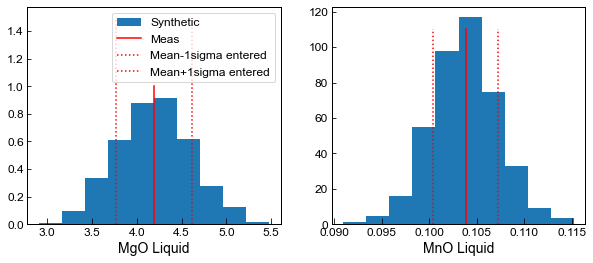
• We can plot some elements up against the user-entered 1 sigma to verify how the code is working

fig, ((ax1, ax2)) = plt.subplots(1, 2, figsize=(10, 4))

ax1.hist(Liquids_only_abs_noise.loc[Liquids_only_abs_noise['Sample_ID_Liq_Num']==0, 'MgO_Liq'],
         label='Synthetic', density=True)  ;
ax1.plot([myLiquids1['MgO_Liq'].iloc[0], myLiquids1['MgO_Liq'].iloc[0]], [0, 1], '-r', label='Meas')
ax1.plot([myLiquids1['MgO_Liq'].iloc[0]-myLiquids1_Err['MgO_Liq_Err'].iloc[0],
          myLiquids1['MgO_Liq'].iloc[0]-myLiquids1_Err['MgO_Liq_Err'].iloc[0]],
         [0, 1.5], ':r', label='Mean-1sigma entered')
ax1.plot([myLiquids1['MgO_Liq'].iloc[0]+myLiquids1_Err['MgO_Liq_Err'].iloc[0],
          myLiquids1['MgO_Liq'].iloc[0]+myLiquids1_Err['MgO_Liq_Err'].iloc[0]],
         [0, 1.5], ':r', label='Mean+1sigma entered')
ax1.set_xlabel('MgO Liquid')
ax1.legend()

ax2.hist(Liquids_only_abs_noise.loc[Liquids_only_abs_noise['Sample_ID_Liq_Num']==0, 'MnO_Liq'],
         label='Synthetic', density=True)  ;
ax2.plot([myLiquids1['MnO_Liq'].iloc[0], myLiquids1['MnO_Liq'].iloc[0]], [0, 110], '-r', label='Ent. Value')
ax2.plot([myLiquids1['MnO_Liq'].iloc[0]-myLiquids1_Err['MnO_Liq_Err'].iloc[0],
          myLiquids1['MnO_Liq'].iloc[0]-myLiquids1_Err['MnO_Liq_Err'].iloc[0]],
         [0, 110], ':r', label='Mean-1sigma entered')
ax2.plot([myLiquids1['MnO_Liq'].iloc[0]+myLiquids1_Err['MnO_Liq_Err'].iloc[0],
          myLiquids1['MnO_Liq'].iloc[0]+myLiquids1_Err['MnO_Liq_Err'].iloc[0]],
         [0, 110], ':r', label='Mean+1sigma entered')
ax2.set_xlabel('MnO Liquid')

Text(0.5, 0, 'MnO Liquid')

Step 2 - input this synthetic dataframe into the functions for calculating temperature

• Here, using equation 22 of Putirka (2008), where DMg ol-liq is calculated theoretically using DMg from Beattie (1993) so this can be used as an olivine-only thermometer

T_noise=pt.calculate_liq_only_temp(liq_comps=Liquids_only_abs_noise, equationT="T_Put2008_eq22_BeattDMg",
                                   P=5)

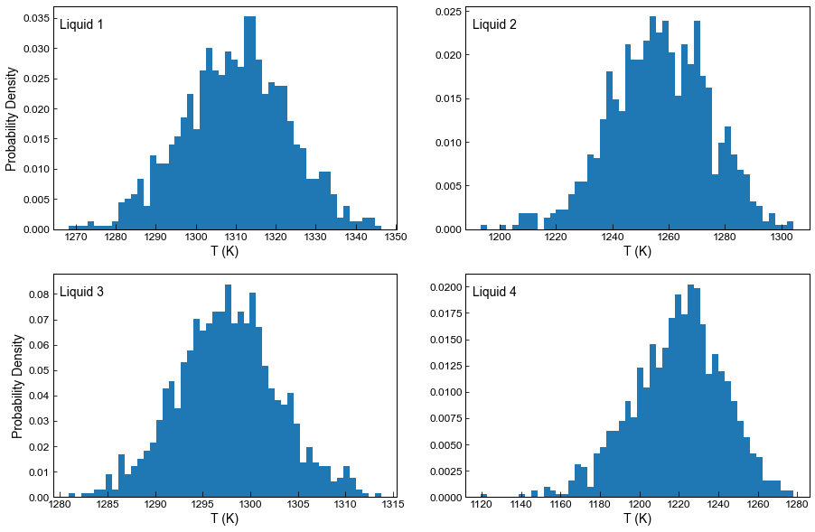
Step 3 - Plot the results

• In this plot we show the histogram for the temperature from each liquid for liquid 1, 2, 3, and 4 (for all 1000 synthetic liquids generated from each measured liquid)

• All synthetic liquids generated from a single input liquid have the same value of ‘Sample_ID_Liq_Num’

fig, ((ax1, ax2), (ax3, ax4)) = plt.subplots(2, 2, figsize=(15, 10))
ax1.annotate("Liquid 1", xy=(0.02, 0.9), xycoords="axes fraction", fontsize=14)
ax1.hist(T_noise.loc[Liquids_only_abs_noise['Sample_ID_Liq_Num']==0], bins=50, density=True);
ax2.annotate("Liquid 2", xy=(0.02, 0.9), xycoords="axes fraction", fontsize=14)
ax2.hist(T_noise.loc[Liquids_only_abs_noise['Sample_ID_Liq_Num']==1], bins=50, density=True);
ax3.annotate("Liquid 3", xy=(0.02, 0.9), xycoords="axes fraction", fontsize=14)
ax3.hist(T_noise.loc[Liquids_only_abs_noise['Sample_ID_Liq_Num']==2], bins=50, density=True);
ax4.annotate("Liquid 4", xy=(0.02, 0.9), xycoords="axes fraction", fontsize=14)
ax4.hist(T_noise.loc[Liquids_only_abs_noise['Sample_ID_Liq_Num']==3], bins=50, density=True);
ax1.set_xlabel('T (K)')
ax2.set_xlabel('T (K)')
ax4.set_xlabel('T (K)')
ax3.set_xlabel('T (K)')
ax1.set_ylabel('Probability Density')
ax3.set_ylabel('Probability Density')

Text(0, 0.5, 'Probability Density')

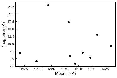
Step 4 - Use a function to get the mean, median and standard deviation for each liquid

The two arguements for this function are:

1. The panda series you want to average (in this case, temperature)

2. The panda series of values you want to average by, e.g., here averaging all samples with the same sample ID.

Stats_T_K=pt.av_noise_samples_series(T_noise, Liquids_only_abs_noise['Sample_ID_Liq_Num'])
Stats_T_K

	Sample	# averaged	Mean_calc	Median_calc	St_dev_calc	St_dev_calc_from_percentiles	Max_calc	Min_calc
0	0.0	1000	1310.325840	1310.922770	12.888252	12.978717	1346.394311	1261.284772
1	1.0	1000	1257.434360	1258.783787	17.097877	16.891889	1305.977173	1193.563542
2	2.0	1000	1297.615797	1297.556694	5.249221	5.360861	1313.397696	1283.195602
3	3.0	1000	1219.564426	1221.374453	23.241533	22.543334	1288.193433	1134.707460
4	4.0	1000	1283.606821	1283.525705	7.138253	7.153480	1306.661208	1264.127265
5	5.0	1000	1269.296891	1269.388903	3.413216	3.350003	1282.305034	1258.529231
6	6.0	1000	1259.313812	1259.338805	5.637615	5.452693	1276.675205	1242.120793
7	7.0	1000	1197.264888	1197.149715	4.218156	4.220776	1211.215580	1184.256181
8	8.0	1000	1167.099056	1167.426108	6.981967	6.912861	1189.721622	1139.965886
9	9.0	1000	1335.282359	1335.246673	8.826425	8.536548	1363.073219	1306.362807

## You can plot these up too
plt.plot(Stats_T_K['Mean_calc'], Stats_T_K['St_dev_calc'], 'ok')
plt.xlabel('Mean T (K)')
plt.ylabel('1 sig error (K)')

Text(0, 0.5, '1 sig error (K)')

Example 2 - Making noise using percentage Errors

• Here, in the input spreadsheet we have specified a percentage error for each input (e.g., you could estimate this from EPMA analyses of secondary standards, or from EPMA software 1 sigma outputs).

out2=pt.import_excel('Liquid_Errors.xlsx', sheet_name="Error_Example_Perc")
my_input2=out2['my_input']
myOls2=out2['Ols']
myLiquids2=out2['Liqs']

out_Err2=pt.import_excel_errors('Liquid_Errors.xlsx', sheet_name="Error_Example_Perc")
myLiquids2_Err=out_Err2['Liqs_Err']
myinput2_Out=out_Err2['my_input_Err']

display(myLiquids2_Err.head())

	SiO2_Liq_Err	TiO2_Liq_Err	Al2O3_Liq_Err	FeOt_Liq_Err	MnO_Liq_Err	MgO_Liq_Err	CaO_Liq_Err	Na2O_Liq_Err	K2O_Liq_Err	Cr2O3_Liq_Err	P2O5_Liq_Err	H2O_Liq_Err	Fe3Fet_Liq_Err	NiO_Liq_Err	CoO_Liq_Err	CO2_Liq_Err	Sample_ID_Liq_Err	P_kbar_Err	T_K_Err
0	1	3	5	4	10	2	3	10	10	20	5	10	0.0	0.0	0.0	0.0	0	1	1
1	1	3	5	4	10	2	3	10	10	20	5	10	0.0	0.0	0.0	0.0	1	1	1
2	1	3	5	4	10	2	3	10	10	20	5	10	0.0	0.0	0.0	0.0	2	1	1
3	1	3	5	4	10	2	3	10	10	20	5	10	0.0	0.0	0.0	0.0	3	1	1
4	1	3	5	4	10	2	3	10	10	20	5	10	0.0	0.0	0.0	0.0	4	1	1

Step 1 - add errors based on the dataframe Liquid2_Err which are percentage errors.

• makes 1000 liquids per user-entered row, and assume errors are normally distributed

• The difference from example 1 is now we say phase_err_type=”Perc” not “Abs”

• Here, say Positive=False, which means it keeps negative numbers

Liquids_only_noise2=pt.add_noise_sample_1phase(phase_comp=myLiquids2, phase_err=myLiquids2_Err,
                     phase_err_type="Perc", duplicates=1000, err_dist="normal", positive=False)

c:\users\penny\box\postdoc\mybarometers\thermobar_outer\src\Thermobar\noise_averaging.py:587: FutureWarning: Downcasting object dtype arrays on .fillna, .ffill, .bfill is deprecated and will change in a future version. Call result.infer_objects(copy=False) instead. To opt-in to the future behavior, set `pd.set_option('future.no_silent_downcasting', True)`
  mynoisedDataframe=mynoisedDataframe.fillna(0)

# Validation that its calculating percentage errors right, as told it to add 1% error for SiO2.
#This will vary a bit as you run it, as its random
Mean=np.mean(Liquids_only_noise2.loc[Liquids_only_noise2['Sample_ID_Liq_Num']==0, 'SiO2_Liq'])
std_Dev=np.nanstd(Liquids_only_noise2.loc[Liquids_only_noise2['Sample_ID_Liq_Num']==0, 'SiO2_Liq'])
100*std_Dev/Mean

1.04939854205056

Step 2 - calculating temperatures for all these synthetic liquids using equation 16 of Putirka (2008)

T_noise2=pt.calculate_liq_only_temp(liq_comps=Liquids_only_noise2, equationT="T_Put2008_eq16", P=5)

Step 3 - Calculating standard deviations, means, and medians etc

Stats_T_K2=pt.av_noise_samples_series(T_noise2, Liquids_only_noise2['Sample_ID_Liq_Num'])
Stats_T_K2

	Sample	# averaged	Mean_calc	Median_calc	St_dev_calc	St_dev_calc_from_percentiles	Max_calc	Min_calc
0	0.0	1000	1360.933884	1360.141582	21.727890	21.205169	1445.503924	1294.701782
1	1.0	1000	1283.483602	1282.334741	24.908077	25.190060	1361.250518	1196.503437
2	2.0	1000	1291.171070	1289.503809	28.172387	27.297823	1387.960527	1212.835111
3	3.0	1000	1262.184145	1261.457359	33.430908	31.982655	1383.533306	1158.523046
4	4.0	1000	1327.911503	1326.994373	17.182505	16.951246	1385.803735	1280.630319
5	5.0	1000	1309.486855	1308.863081	18.816263	18.364905	1376.596055	1250.606787
6	6.0	1000	1292.310744	1292.742919	22.452813	21.590959	1388.051709	1224.410309
7	7.0	1000	1375.866861	1375.618995	18.015605	18.111736	1435.328225	1325.458581
8	8.0	1000	1280.264848	1279.260695	21.312228	21.541613	1343.011630	1224.618223
9	9.0	1000	1381.730332	1381.445031	11.914272	11.541467	1423.635066	1347.053781

Example 3: Fixed Percentage Error

• Here, instead of inputted columns with “_Err” for each oxide, we just add a fixed percentage error to all oxides (still normally distributed) - here, 1% noise for all elements

out3=pt.import_excel('Liquid_Errors.xlsx', sheet_name="Error_Example_Perc")
my_input3=out3['my_input']
myOls23=out3['Ols']
myLiquids3=out3['Liqs']

Liquids_only_noise3=pt.add_noise_sample_1phase(phase_comp=myLiquids3, duplicates=1000,
                           noise_percent=1, err_dist="normal")

All negative numbers replaced with zeros. If you wish to keep these, set positive=False

T_noise3=pt.calculate_liq_only_temp(liq_comps=Liquids_only_noise3, equationT="T_Put2008_eq16", P=5)

Stats_T_K3=pt.av_noise_samples_series(T_noise3, Liquids_only_noise3['Sample_ID_Liq_Num'])
Stats_T_K3

	Sample	# averaged	Mean_calc	Median_calc	St_dev_calc	St_dev_calc_from_percentiles	Max_calc	Min_calc
0	0.0	1000	1361.120327	1361.102666	4.962582	4.764748	1379.980257	1344.369392
1	1.0	1000	1283.832846	1283.763313	5.738179	5.626146	1302.340045	1266.417632
2	2.0	1000	1289.454109	1289.308731	6.276238	6.234107	1314.591478	1271.960229
3	3.0	1000	1263.267406	1262.957989	7.517084	7.107076	1286.982196	1242.571952
4	4.0	1000	1327.366378	1327.321600	3.582536	3.494084	1341.622115	1317.152343
5	5.0	1000	1310.400864	1310.396428	4.197083	4.240772	1325.117670	1296.155068
6	6.0	1000	1292.050325	1291.979601	4.679050	4.821711	1306.300090	1276.171300
7	7.0	1000	1376.055416	1375.946298	4.269935	4.043297	1393.749359	1363.273474
8	8.0	1000	1279.536538	1279.503841	4.446930	4.438310	1294.552032	1263.699851
9	9.0	1000	1381.084674	1381.126509	2.890563	2.904920	1389.509444	1371.026061

Example 4: Perc uncertainty in a single input parameter

• Here, want to add 5% error to just MgO in the liquid. You don’t have to specify _Liq, it adds this based on what you entered.

Liquids_only_noise4=pt.add_noise_sample_1phase(phase_comp=myLiquids1, variable="MgO", variable_err=5,
                                              variable_err_type="Perc", duplicates=1000, err_dist="normal")

All negative numbers replaced with zeros. If you wish to keep these, set positive=False

T_noise4=pt.calculate_liq_only_temp(liq_comps=Liquids_only_noise4, equationT="T_Put2008_eq16", P=5)

Stats_T_K4=pt.av_noise_samples_series(T_noise4, Liquids_only_noise4['Sample_ID_Liq_Num'])
Stats_T_K4

	Sample	# averaged	Mean_calc	Median_calc	St_dev_calc	St_dev_calc_from_percentiles	Max_calc	Min_calc
0	0.0	1000	1361.115535	1360.940344	6.400013	6.418018	1380.459533	1340.910519
1	1.0	1000	1283.562104	1283.524037	5.091750	5.180471	1306.786283	1268.778112
2	2.0	1000	1289.371106	1289.514375	4.531075	4.587816	1303.324783	1272.753201
3	3.0	1000	1262.632158	1262.702508	3.285891	3.352616	1271.546811	1252.490440
4	4.0	1000	1327.293664	1327.443628	6.583046	6.418376	1346.807116	1305.553288
5	5.0	1000	1310.219435	1309.923383	5.788320	5.757229	1328.997356	1288.443216
6	6.0	1000	1291.971382	1292.070215	4.818476	4.659367	1305.010246	1276.820791
7	7.0	1000	1375.551449	1375.642808	7.366337	7.479750	1396.361262	1352.664779
8	8.0	1000	1279.523343	1279.674720	6.777822	6.902977	1300.817787	1259.625361
9	9.0	1000	1380.838405	1380.834433	8.198617	8.587369	1405.100823	1355.972728

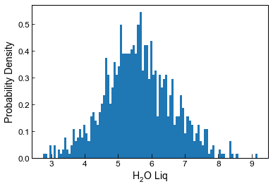
Example 5: Absolute uncertainty in a given input parameter

• Here, say uncertainty in H2O content of the liquid is +-1 wt%

Liquids_only_noise5=pt.add_noise_sample_1phase(phase_comp=myLiquids1, variable="H2O", variable_err=1,
                                              variable_err_type="Abs", duplicates=1000, err_dist="normal")

All negative numbers replaced with zeros. If you wish to keep these, set positive=False

plot a histogram of resulting H2O distribution

plt.hist(Liquids_only_noise5.loc[Liquids_only_noise4['Sample_ID_Liq_Num']==0, 'H2O_Liq'], bins=100, density= True);
plt.xlabel('H$_2$O Liq')
plt.ylabel('Probability Density')

Text(0, 0.5, 'Probability Density')

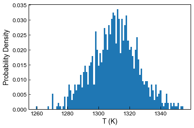
Now feed this into a thermometer

#Feed into a thermometer
T_noise5=pt.calculate_liq_only_temp(liq_comps=Liquids_only_noise5, equationT="T_Put2008_eq22_BeattDMg",
                              P=5)
plt.hist(T_noise5.loc[Liquids_only_noise5['Sample_ID_Liq_Num']==0], bins=100, density=True);
plt.ylabel('Probability Density')
plt.xlabel('T (K)')

Text(0.5, 0, 'T (K)')

Stats_T_K5=pt.av_noise_samples_series(T_noise5, Liquids_only_noise5['Sample_ID_Liq_Num'])
Stats_T_K5

	Sample	# averaged	Mean_calc	Median_calc	St_dev_calc	St_dev_calc_from_percentiles	Max_calc	Min_calc
0	0.0	1000	1311.147914	1310.648202	14.699344	15.172898	1355.014277	1268.311283
1	1.0	1000	1257.865317	1257.297150	13.579432	14.110573	1296.963638	1207.760993
2	2.0	1000	1297.270728	1296.667132	14.639945	13.913746	1344.062283	1246.906532
3	3.0	1000	1221.480365	1220.853754	12.393805	12.238216	1263.319981	1183.676652
4	4.0	1000	1282.783994	1283.259223	13.699640	13.509715	1323.330615	1238.148956
5	5.0	1000	1269.745910	1269.360221	13.944938	13.816489	1317.958573	1224.615807
6	6.0	1000	1259.986365	1259.339462	13.813587	13.476064	1298.209774	1219.803599
7	7.0	1000	1196.783075	1196.709610	11.998598	11.951581	1233.626161	1156.211936
8	8.0	1000	1167.055980	1166.579713	11.405290	11.236524	1201.954372	1124.707021
9	9.0	1000	1335.012077	1334.823792	15.552100	15.201209	1378.484958	1285.601887

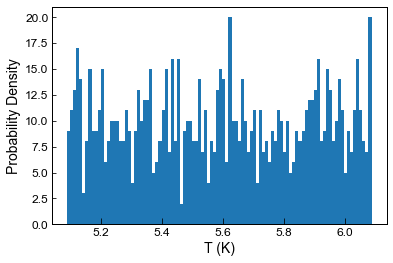
Example 6 - Uniformly distributed errors

• by default, the code assumes a normal distribution of errors, calculated using the user-inputted 1 sigma value

• you can also state err_dist=”uniform”, to generate uniformly distributed noise between +-inputted value

Liquids_only_noise6=pt.add_noise_sample_1phase(phase_comp=myLiquids1, variable="H2O", variable_err=0.5,
                                              variable_err_type="Abs", duplicates=1000, err_dist="uniform")

All negative numbers replaced with zeros. If you wish to keep these, set positive=False

plt.hist(Liquids_only_noise6.loc[Liquids_only_noise6['Sample_ID_Liq_Num']==0, 'H2O_Liq'], bins=100);
plt.ylabel('Probability Density')
plt.xlabel('T (K)')

Text(0.5, 0, 'T (K)')