This page was generated from docs/Examples/Error_propagation/Cpx_only_contour_plot.ipynb. Interactive online version: .

Python Notebook Download

Error propagation - Cpx-only

• This notebook gives a worked example showing how to propagate uncertainty for Cpx-only thermometry for different amounts of EPMA-based error on Na\(_2\)O measurements.

• We use the functionality provided by Pyrolite to contour the results from Monte Carlo simulations, as well as hexplot.

• If you use the pyroplot.density command, please remember to cite Pyrolite! (Williams et al., (2020). pyrolite: Python for geochemistry. Journal of Open Source Software, 5(50), 2314, doi: 10.21105/joss.02314)

• This builds on from the notebook showing how to consider error in a single phase (Liquid_Thermometry_error_prop.ipynb). We suggest you look at that first, as its simpler when you don’t have to worry about two separate phases

• We consider an example Cpx composition from Gleeson et al. (2020) - https://doi.org/10.1093/petrology/egaa094

• You can download the Excel spreadsheet here: https://github.com/PennyWieser/Thermobar/blob/main/docs/Examples/Error_propagation/Gleeson2020_Cpx_Comps.xlsx

You need to install Thermobar once on your machine, if you haven’t done this yet, uncomment the line below (remove the #)

#!pip install Thermobar

You will also need to install pyrolite for this example, if you haven’t done so already, uncomment the line below

#!pip install pyrolite

# Import other python stuff
import numpy as np
import pandas as pd
import matplotlib.pyplot as plt
import Thermobar as pt
import sympy as sym
pd.options.display.max_columns = None
import pyrolite

Importing data

• Note, we haven’t bothered to add the “_Cpx” names after each oxide, so we simply use “suffix=”_Cpx” when we load the data

out=pt.import_excel('Gleeson2020_Cpx_Comps.xlsx', sheet_name="Sheet1", suffix="_Cpx")
my_input=out['my_input']
myCpxs1=out['Cpxs']

Lets select 1 Cpx to run the calculations on

• The [[ ]] keeps it as a dataframe

myCpxs1.iloc[[0]]

	SiO2_Cpx	TiO2_Cpx	Al2O3_Cpx	FeOt_Cpx	MnO_Cpx	MgO_Cpx	CaO_Cpx	Na2O_Cpx	K2O_Cpx	Cr2O3_Cpx	Sample_ID_Cpx
0	51.3863	0.467	4.1961	3.8654	0.12	16.3137	21.3039	0.378	0.0007	1.0191	0

Work out errors

• The Cameca software used to analyse these Cpxs returns the error as absolute elemental wt%, ignoring Oxygen, for each element (helpful!). These are loaded in as Na_Err, Si_Err….

• This means that you need to do some steps to work out the analytical error on each Cpx. We show these steps below.

• First, we decide it easiest to use the convert_oxide_percent_to_element_weight_percent function to convert measured Cpx compositions as oxides into wt% to compare to these errors. Without oxygen = True, does the calculations without oxygen. You can use this function for any phase, just specify what suffix your phase has.

Cpx_conv=pt.convert_oxide_percent_to_element_weight_percent(df=myCpxs1, suffix='_Cpx', without_oxygen=True)
Cpx_conv.head()

	Si_wt_noO2	Mg_wt_noO2	Fe_wt_noO2	Ca_wt_noO2	Al_wt_noO2	Na_wt_noO2	K_wt_noO2	Mn_wt_noO2	Ti_wt_noO2	Cr_wt_noO2	P_wt_noO2	F_wt_noO2	H_wt_noO2	Cl_wt_noO2
0	43.155184	17.675115	5.398069	27.354400	3.989980	0.503819	0.001044	0.166972	0.502666	1.252750	0.0	0.0	0.0	0.0
1	42.432683	17.004438	5.468846	27.558497	4.967044	0.507369	0.000447	0.121440	0.625890	1.313346	0.0	0.0	0.0	0.0
2	42.399838	16.694183	5.608834	27.398388	5.209677	0.523472	0.022141	0.141541	0.681296	1.320631	0.0	0.0	0.0	0.0
3	42.649103	17.224819	5.638033	27.496627	4.631102	0.538772	0.004336	0.097927	0.632681	1.086601	0.0	0.0	0.0	0.0
4	41.057438	15.479289	7.324030	26.604851	6.874709	0.702197	0.025343	0.188588	1.005908	0.737648	0.0	0.0	0.0	0.0

• Now we calculate the % error for each element. For example, for Na, we take the Cameca error (column Na_Err), and compare it to the concentration we just calculated in wt% for Na (column Na_wt_noO2 in the Cpx_conv dataframe)

Perc_Err_Na=100*my_input['Na_Err']/Cpx_conv['Na_wt_noO2']
Perc_Err_Na.head()

0    8.534819
1    8.553938
2    8.520041
3    8.315210
4    7.049307
dtype: float64

# We now need to re-arrange these into a form that we can load into the function.
# We make a new dataframe of these errors
df_Cpx_Err=pd.DataFrame(data={'SiO2_Cpx_Err': 100*my_input['Si_Err']/Cpx_conv['Si_wt_noO2'],
                            'TiO2_Cpx_Err':100*my_input['Ti_Err']/Cpx_conv['Ti_wt_noO2'],
                             'Al2O3_Cpx_Err':100*my_input['Al_Err']/Cpx_conv['Al_wt_noO2'],
                             'FeOt_Cpx_Err':100*my_input['Fe_Err']/Cpx_conv['Fe_wt_noO2'],
                            'MnO_Cpx_Err':100*my_input['Mn_Err']/Cpx_conv['Mn_wt_noO2'],
                            'MgO_Cpx_Err':100*my_input['Mg_Err']/Cpx_conv['Mg_wt_noO2'],
                            'CaO_Cpx_Err':100*my_input['Ca_Err']/Cpx_conv['Ca_wt_noO2'],
                            'Na2O_Cpx_Err':100*my_input['Na_Err']/Cpx_conv['Na_wt_noO2'],
                            'Cr2O3_Cpx_Err':100*my_input['Cr_Err']/Cpx_conv['Cr_wt_noO2'],
                               'K2O_Cpx_Err': 100*my_input['K_Err']/Cpx_conv['K_wt_noO2']}, index=[0])

Lets select 1 Cpx, and its corresponding error as an example

• using [[ ]] keeps it as a dataframe, we reset the index because sometimes this can cause python mayhem.

Cpx_1=myCpxs1.iloc[[0]].reset_index(drop=True)
Cpx_1_Err=df_Cpx_Err.iloc[[0]].reset_index(drop=True)
Cpx_1_Err

	SiO2_Cpx_Err	TiO2_Cpx_Err	Al2O3_Cpx_Err	FeOt_Cpx_Err	MnO_Cpx_Err	MgO_Cpx_Err	CaO_Cpx_Err	Na2O_Cpx_Err	Cr2O3_Cpx_Err	K2O_Cpx_Err
0	1.186416	2.148544	0.907273	3.056648	27.309951	1.129271	0.858363	8.534819	5.172622	1934.77739

Lets calculate the errors for this Cpx

• You could do this for all Cpxs, rather than just this 1 sample, but it’ll take longer, so we do a cut down version here!

• 20,000 iterations may seem like a lot, but it really helps with the contouring

Calc_Cpx_dist=pt.add_noise_sample_1phase(phase_comp=Cpx_1, phase_err=Cpx_1_Err,
                                            phase_err_type="Perc", duplicates=20000, err_dist="normal")

All negative numbers replaced with zeros. If you wish to keep these, set positive=False

Lets calculate pressures and temperatures using a wide variety of equations for Cpx-only thermobarometry

• This cell takes abit of time, its 20,000 calculations using a wide variety of P and T equations!

Calc_PT=pt.calculate_cpx_only_press_all_eqs(cpx_comps=Calc_Cpx_dist)
Calc_PT.head()

---------------------------------------------------------------------------
ValueError                                Traceback (most recent call last)
c:\Users\penny\Box\Postdoc\MyBarometers\Thermobar_outer\docs\Examples\Error_propagation\Cpx_only_contour_plot.ipynb Cell 21 line 1
----> <a href='vscode-notebook-cell:/c%3A/Users/penny/Box/Postdoc/MyBarometers/Thermobar_outer/docs/Examples/Error_propagation/Cpx_only_contour_plot.ipynb#X26sZmlsZQ%3D%3D?line=0'>1</a> Calc_PT=pt.calculate_cpx_only_press_all_eqs(cpx_comps=Calc_Cpx_dist)
      <a href='vscode-notebook-cell:/c%3A/Users/penny/Box/Postdoc/MyBarometers/Thermobar_outer/docs/Examples/Error_propagation/Cpx_only_contour_plot.ipynb#X26sZmlsZQ%3D%3D?line=1'>2</a> Calc_PT.head()

File c:\users\penny\box\postdoc\mybarometers\thermobar_outer\src\Thermobar\clinopyroxene_thermobarometry.py:3365, in calculate_cpx_only_press_all_eqs(cpx_comps, plot, return_cpx, H2O_Liq)
   3360 cpx_comps_c['T_Wang21_eq2']=calculate_cpx_only_temp(cpx_comps=cpx_comps_copy, equationT="T_Wang2021_eq2", H2O_Liq=H2O_Liq)
   3362 cpx_comps_c['T_Petrelli20']=calculate_cpx_only_temp(cpx_comps=cpx_comps_copy,
   3363 equationT="T_Petrelli2020_Cpx_only_onnx")
-> 3365 cpx_comps_c['T_Jorgenson22']=calculate_cpx_only_temp(cpx_comps=cpx_comps_copy,
   3366 equationT="T_Jorgenson2022_Cpx_only_onnx")
   3368 # cpx_comps_c['T_Petrelli21_H2O']=calculate_cpx_only_temp(cpx_comps=cpx_comps_copy,
   3369 # equationT="T_Petrelli2020_Cpx_only_withH2O_onnx").T_K_calc
   3370 #
   3371 # cpx_comps_c['P_Petrelli21_H2O']=calculate_cpx_only_press(cpx_comps=cpx_comps_copy,
   3372 # equationP="P_Petrelli2020_Cpx_only_withH2O").P_kbar_calc
   3374 cpx_comps_c['T_Put_Teq32d_Peq32a']=calculate_cpx_only_press_temp(cpx_comps=cpx_comps_copy,
   3375 equationP="P_Put2008_eq32a", equationT="T_Put2008_eq32d").T_K_calc

File c:\users\penny\box\postdoc\mybarometers\thermobar_outer\src\Thermobar\clinopyroxene_thermobarometry.py:3537, in calculate_cpx_only_temp(cpx_comps, equationT, P, H2O_Liq, eq_tests)
   3533     T_K=df_stats['T_K_calc']
   3535 elif ('Petrelli' in equationT or "Jorgenson" in equationT) and "onnx" in equationT:
-> 3537     T_K=func(cpx_comps=cpx_comps_c)
   3541 else:
   3543     kwargs = {name: cpx_components[name] for name, p in sig.parameters.items()
   3544     if p.kind == inspect.Parameter.KEYWORD_ONLY}

File c:\users\penny\box\postdoc\mybarometers\thermobar_outer\src\Thermobar\clinopyroxene_thermobarometry.py:1769, in T_Jorgenson2022_Cpx_only_onnx(P, cpx_comps)
   1767 import onnxruntime as rt
   1768 path=Path(Thermobar_onnx.__file__).parent
-> 1769 sess =  rt.InferenceSession(str(path/"Jorg21_Cpx_only_Temp.onnx"))
   1772 input_name = sess.get_inputs()[0].name
   1773 label_name = sess.get_outputs()[0].name

File c:\Users\penny\anaconda3\Lib\site-packages\onnxruntime\capi\onnxruntime_inference_collection.py:432, in InferenceSession.__init__(self, path_or_bytes, sess_options, providers, provider_options, **kwargs)
    430         raise fallback_error from e
    431 # Fallback is disabled. Raise the original error.
--> 432 raise e

File c:\Users\penny\anaconda3\Lib\site-packages\onnxruntime\capi\onnxruntime_inference_collection.py:419, in InferenceSession.__init__(self, path_or_bytes, sess_options, providers, provider_options, **kwargs)
    416 disabled_optimizers = kwargs["disabled_optimizers"] if "disabled_optimizers" in kwargs else None
    418 try:
--> 419     self._create_inference_session(providers, provider_options, disabled_optimizers)
    420 except (ValueError, RuntimeError) as e:
    421     if self._enable_fallback:

File c:\Users\penny\anaconda3\Lib\site-packages\onnxruntime\capi\onnxruntime_inference_collection.py:451, in InferenceSession._create_inference_session(self, providers, provider_options, disabled_optimizers)
    449 if not providers and len(available_providers) > 1:
    450     self.disable_fallback()
--> 451     raise ValueError(
    452         f"This ORT build has {available_providers} enabled. "
    453         "Since ORT 1.9, you are required to explicitly set "
    454         "the providers parameter when instantiating InferenceSession. For example, "
    455         f"onnxruntime.InferenceSession(..., providers={available_providers}, ...)"
    456     )
    458 session_options = self._sess_options if self._sess_options else C.get_default_session_options()
    459 if self._model_path:

ValueError: This ORT build has ['AzureExecutionProvider', 'CPUExecutionProvider'] enabled. Since ORT 1.9, you are required to explicitly set the providers parameter when instantiating InferenceSession. For example, onnxruntime.InferenceSession(..., providers=['AzureExecutionProvider', 'CPUExecutionProvider'], ...)

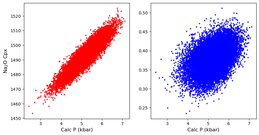
Lets plot these calculations using the Wang et al. (2021) thermometer and barometer

• You can see that despite random input errors, P and T end up correlated in the resulting distribution

• You can also see that pressure is controlled predominantly by the error on the Na2O component, with scatter around this trend

fig, (ax1, ax2) = plt.subplots(1, 2, figsize=(10,5))
ax1.plot(Calc_PT['P_Wang21_eq1'], Calc_PT['T_Wang21_eq2'], '.r' )
ax2.plot(Calc_PT['P_Wang21_eq1'], Calc_PT['Na2O_Cpx'], '.b' )
ax1.set_xlabel('Calc P (kbar)')
ax2.set_xlabel('Calc P (kbar)')
ax1.set_ylabel('Calc T (K)')
ax1.set_ylabel('Na$_2$O Cpx')

Text(0, 0.5, 'Na$_2$O Cpx')

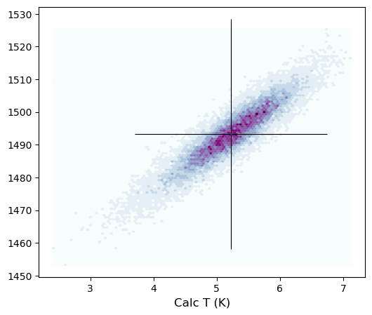
A more robust way to show this

• If you play around with duplicates = , you’ll see that the more points you ask for, the more spread in pressure space.

• It is more robust to contour results

• First, we show how to do this using hexbin (matplotlib)

• We underlie the published error on the barometer, at the average calculated composition.

fig, (ax1)  = plt.subplots(1, 1, figsize=(6,5))

ax1.hexbin(Calc_PT['P_Wang21_eq1'],
           Calc_PT['T_Wang21_eq2'],
            cmap=plt.cm.BuPu,
            linewidths=0.2, bins=10)
ax1.set_xlabel('Calc P (kbar)')
ax1.set_xlabel('Calc T (K)')


ax1.errorbar(np.mean(Calc_PT['P_Wang21_eq1']),
             np.mean(Calc_PT['T_Wang21_eq2']),
             xerr=1.52, yerr=35.2,
             fmt='.', ecolor='k', elinewidth=0.8, mfc='k', ms=1)

<ErrorbarContainer object of 3 artists>

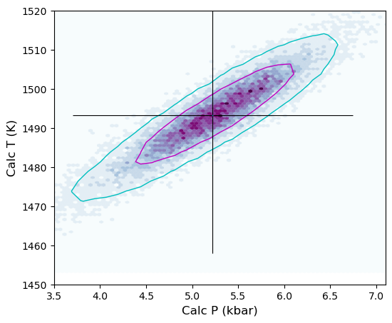
But this is still hard to visualize!

• We can add contours using pyrolite, so we can visualize where 67% of simulations lie, and where 95% of simulations lie

• You will have to play around a bit with the number of bins, and the extent parameter.

• We always plot PT first, then use that to work out the extent, which tells the code where to look for contours in. This only needs to be approximate.

• This step can be slow, if you are using 4-8 Gb of Ram, you might want to reduce the number of duplicates when you make the samples.

• Remember to cite Pyrolite if you use these contours!

fig, (ax1)  = plt.subplots(1, 1, figsize=(6,5))

# This parameter helps pyrolite converge on the contour positions faster,
# e.g. saying look for contours between 3.5 and 7 kbar
# and between 1470 and 1540 K. You'll need to change this for your particular system
extent1=(3.5, 7, 1470, 1540)
ax1.hexbin(Calc_PT['P_Wang21_eq1'],
           Calc_PT['T_Wang21_eq2'],
            cmap=plt.cm.BuPu,
            linewidths=0.2, bins=10)
ax1.set_xlabel('Calc P (kbar)')
ax1.set_xlabel('Calc T (K)')


Calc_PT.loc[:,
["P_Wang21_eq1", "T_Wang21_eq2"]].pyroplot.density(ax=ax1, contours=[0.67, 0.95], colors=['m', 'c'],
                                                   extent=extent1, cmap="viridis",
                                                   bins=30, label_contours=False)
# Adjust axes limits
ax1.set_xlim([3.5, 7.1])
ax1.set_ylim([1450,  1520])

ax1.errorbar(np.mean(Calc_PT['P_Wang21_eq1']),
             np.mean(Calc_PT['T_Wang21_eq2']),
             xerr=1.52, yerr=35.2,
             fmt='.', ecolor='k', elinewidth=0.8, mfc='k', ms=1)

ax1.set_xlabel('Calc P (kbar)')
ax1.set_ylabel('Calc T (K)')

Text(0, 0.5, 'Calc T (K)')

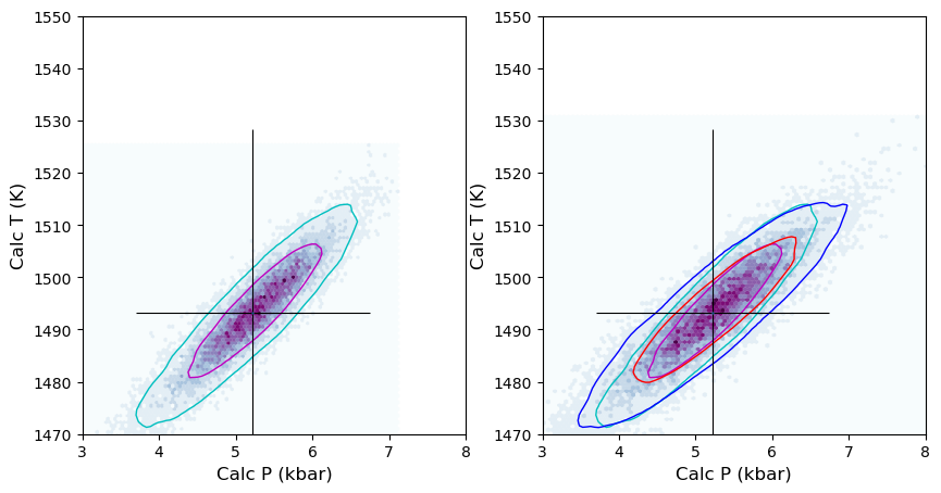
Lets work out what would happen if we doubled the analytical error on Na2O

• Be patient, this takes a bit of time, its 20,000 calculations!

# First, lets duplicate the error dataframe
df_Cpx_Err_2Na=df_Cpx_Err.copy()
# Lets set Na2O error to 2* what it was
df_Cpx_Err_2Na['Na2O_Cpx_Err']=2*df_Cpx_Err['Na2O_Cpx_Err']
# And lets take sample 0 again
Cpx_1_Err_2Na=df_Cpx_Err_2Na.iloc[[0]].reset_index(drop=True)
# Lets simulate some new Cpxs.
Calc_Cpx_dist_2Na=pt.add_noise_sample_1phase(phase_comp=Cpx_1, phase_err=Cpx_1_Err_2Na,
                                             phase_err_type="Perc", duplicates=20000, err_dist="normal")
# And lets calculate pressures
Calc_PT_2Na=pt.calculate_cpx_only_press_all_eqs(cpx_comps=Calc_Cpx_dist_2Na)

All negative numbers replaced with zeros. If you wish to keep these, set positive=False

Lets plot these new errors vs. the old errors

• Again, the contours can take ~30s to appear (with 16 Gb of RAM)

fig, (ax1, ax2)  = plt.subplots(1, 2, figsize=(10,5), sharex=True, sharey=True)


extent1=(3.5, 7, 1470, 1540)
ax1.hexbin(Calc_PT['P_Wang21_eq1'],
           Calc_PT['T_Wang21_eq2'],
            cmap=plt.cm.BuPu,
            linewidths=0.2, bins=10)
ax1.set_xlabel('Calc P (kbar)')
ax1.set_xlabel('Calc T (K)')




extent2=(3.5, 7, 1470, 1540)
ax2.hexbin(Calc_PT_2Na['P_Wang21_eq1'],
           Calc_PT_2Na['T_Wang21_eq2'],
            cmap=plt.cm.BuPu,
            linewidths=0.2, bins=10)
ax2.set_xlabel('Calc P (kbar)')
ax2.set_xlabel('Calc T (K)')


Calc_PT.loc[:,
["P_Wang21_eq1", "T_Wang21_eq2"]].pyroplot.density(ax=ax1, contours=[0.67, 0.95], colors=['m', 'c'],
                                                   extent=extent1, cmap="viridis",
                                                   bins=70, label_contours=False)

Calc_PT.loc[:,
["P_Wang21_eq1", "T_Wang21_eq2"]].pyroplot.density(ax=ax2, contours=[0.67, 0.95], colors=['m', 'c'],
                                                   extent=extent1, cmap="viridis",
                                                   bins=70, label_contours=False, width=0.5)

Calc_PT_2Na.loc[:,
["P_Wang21_eq1", "T_Wang21_eq2"]].pyroplot.density(ax=ax2, contours=[0.67, 0.95], colors=['r', 'blue'],
                                                   extent=extent2, cmap="viridis",
                                                   bins=70, label_contours=False)

ax1.errorbar(np.mean(Calc_PT['P_Wang21_eq1']),
             np.mean(Calc_PT['T_Wang21_eq2']),
             xerr=1.52, yerr=35.2,
             fmt='.', ecolor='k', elinewidth=0.8, mfc='k', ms=1)

ax2.errorbar(np.mean(Calc_PT['P_Wang21_eq1']),
             np.mean(Calc_PT['T_Wang21_eq2']),
             xerr=1.52, yerr=35.2,
             fmt='.', ecolor='k', elinewidth=0.8, mfc='k', ms=1)

ax1.set_xlim([3, 8])
ax1.set_ylim([1470,  1550])

ax1.set_xlabel('Calc P (kbar)')
ax1.set_ylabel('Calc T (K)')

ax2.set_xlabel('Calc P (kbar)')
ax2.set_ylabel('Calc T (K)')
ax2.yaxis.set_tick_params(which='both', labelbottom=True)

C:\Users\penny\anaconda3\lib\site-packages\pyrolite\util\plot\density.py:202: UserWarning: The following kwargs were not used by contour: 'width'
  cs = contour(

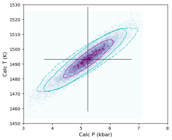
Lets make a pretty figure for publication with just the stated errors for Wang and Putirka thermobarometers, but overlay an additional contour for bigger Na2O errors

# Wang thermobarometers
fig, (ax1)  = plt.subplots(1, figsize=(6,5), sharex=True, sharey=True)

## LHS, Wang et al. 2021
extent1=(3.5, 7, 1470, 1540)
ax1.hexbin(Calc_PT['P_Wang21_eq1'],
           Calc_PT['T_Wang21_eq2'],
            cmap=plt.cm.BuPu,
            linewidths=0.2, bins=10)
ax1.set_xlabel('Calc P (kbar)')
ax1.set_xlabel('Calc T (K)')


Calc_PT.loc[:,
["P_Wang21_eq1", "T_Wang21_eq2"]].pyroplot.density(ax=ax1, contours=[0.67, 0.95], colors=['m', 'c'],
                                                   extent=extent1, cmap="viridis",
                                                   bins=70, label_contours=False)


Calc_PT_2Na.loc[:,
["P_Wang21_eq1", "T_Wang21_eq2"]].pyroplot.density(ax=ax1, contours=[0.95], colors=['c'],
                                                   extent=extent2, cmap="viridis",
                                                   bins=70, label_contours=False,
                                                  linestyles=['-.'])

ax1.errorbar(np.mean(Calc_PT['P_Wang21_eq1']),
             np.mean(Calc_PT['T_Wang21_eq2']),
             xerr=1.52, yerr=35.2,
             fmt='.', ecolor='k', elinewidth=0.8, mfc='k', ms=1)


ax1.set_xlim([3, 8])
ax1.set_ylim([1450,  1530])

ax1.set_xlabel('Calc P (kbar)')
ax1.set_ylabel('Calc T (K)')

ax2.set_xlabel('Calc P (kbar)')
ax2.set_ylabel('Calc T (K)')

ax2.yaxis.set_tick_params(which='both', labelbottom=True)
fig.savefig('Cpx_only_Error.png', dpi=200)

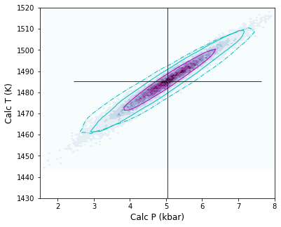
# Putirka Cpx-only barometers
fig, (ax1)  = plt.subplots(1, figsize=(6,5), sharex=True, sharey=True)

## LHS, Wang et al. 2021
extent1=(1, 10, 1430, 1540)
ax1.hexbin(Calc_PT['P_Put_Teq32d_Peq32b'],
           Calc_PT['T_Put_Teq32d_Peq32b'],
            cmap=plt.cm.BuPu,
            linewidths=0.2, bins=10)
ax1.set_xlabel('Calc P (kbar)')
ax1.set_xlabel('Calc T (K)')


Calc_PT.loc[:,
["P_Put_Teq32d_Peq32b", "T_Put_Teq32d_Peq32b"]].pyroplot.density(ax=ax1, contours=[0.67, 0.95], colors=['m', 'c'],
                                                   extent=extent1, cmap="viridis",
                                                   bins=70, label_contours=False)

extent2=(1, 10, 1430, 1540)

Calc_PT_2Na.loc[:,
["P_Put_Teq32d_Peq32b", "T_Put_Teq32d_Peq32b"]].pyroplot.density(ax=ax1, contours=[0.95], colors=['c'],
                                                   extent=extent2, cmap="viridis",
                                                   bins=70, label_contours=False,
                                                  linestyles=['-.'])

ax1.errorbar(np.mean(Calc_PT['P_Put_Teq32d_Peq32b']),
             np.mean(Calc_PT['T_Put_Teq32d_Peq32b']),
             xerr=2.6, yerr=58,
             fmt='.', ecolor='k', elinewidth=0.8, mfc='k', ms=1)


ax1.set_xlim([1.5, 8])
ax1.set_ylim([1430,  1520])

ax1.set_xlabel('Calc P (kbar)')
ax1.set_ylabel('Calc T (K)')

ax2.set_xlabel('Calc P (kbar)')
ax2.set_ylabel('Calc T (K)')

ax2.yaxis.set_tick_params(which='both', labelbottom=True)
fig.savefig('Cpx_only_Error_Put.png', dpi=200)

Lets calculate the statistics for various noise simulations

Stats_P=pt.av_noise_samples_series(Calc_PT['P_Wang21_eq1'], Calc_PT['Sample_ID_Cpx_Num'])
Stats_P

	Sample	Mean_calc	Median_calc	St_dev_calc	Max_calc	Min_calc
0	0.0	5.212426	5.237335	0.576768	7.262507	2.351651

Stats_T=pt.av_noise_samples_series(Calc_PT['T_Wang21_eq2'], Calc_PT['Sample_ID_Cpx_Num'])
Stats_T

	Sample	Mean_calc	Median_calc	St_dev_calc	Max_calc	Min_calc
0	0.0	1493.025062	1493.198869	8.540826	1522.1718	1452.932404

Stats_T=pt.av_noise_samples_series(Calc_PT_2Na['T_Wang21_eq2'], Calc_PT_2Na['Sample_ID_Cpx_Num'])
Stats_T

	Sample	Mean_calc	Median_calc	St_dev_calc	Max_calc	Min_calc
0	0.0	1493.363786	1493.548499	9.11549	1529.575166	1456.638437

Stats_P=pt.av_noise_samples_series(Calc_PT_2Na['P_Wang21_eq1'], Calc_PT_2Na['Sample_ID_Cpx_Num'])
Stats_P

	Sample	Mean_calc	Median_calc	St_dev_calc	Max_calc	Min_calc
0	0.0	5.2346	5.242048	0.714344	8.348103	2.126887

Stats_P_Put=pt.av_noise_samples_series(Calc_PT_2Na['P_Put_Teq32d_Peq32b'], Calc_PT_2Na['Sample_ID_Cpx_Num'])
Stats_P_Put

	Sample	Mean_calc	Median_calc	St_dev_calc	Max_calc	Min_calc
0	0.0	5.013051	5.022533	0.944134	8.845332	0.948181

Stats_P_Put=pt.av_noise_samples_series(Calc_PT['P_Put_Teq32d_Peq32b'], Calc_PT['Sample_ID_Cpx_Num'])
Stats_P_Put

	Sample	Mean_calc	Median_calc	St_dev_calc	Max_calc	Min_calc
0	0.0	5.019986	5.025435	0.83673	8.116579	1.594801

Stats_P_Put=pt.av_noise_samples_series(Calc_PT['T_Put_Teq32d_Peq32b'], Calc_PT['Sample_ID_Cpx_Num'])
Stats_P_Put

	Sample	Mean_calc	Median_calc	St_dev_calc	Max_calc	Min_calc
0	0.0	1485.050547	1485.152212	9.505677	1518.411815	1446.638034