This page was generated from
docs/Examples/Cpx_Cpx_Liq_Thermobarometry/Cpx_Liquid_melt_matching/Cpx_MeltMatch2_ScruggsPutirka2018.ipynb.
Interactive online version:
![]() .
.
This code is a more advanced example of Cpx-Liquid melt matching
It adapts the approach of Scruggs and Putirka, 2018 (https://doi.org/10.2138/am-2018-6058), where you have lots of whole rock compositions for basalts, lots for rhyolites, but nothing in between.
It uses a variety of mixing and sampling algorithms to add “synthetic liquids” you can the feed into the melt matching algoorithm
We suggest you first go through the Cpx_MeltMatch1_Gleeson2020 tutorial for an introduction to the melt matching code
You can download the required excel spreadsheet from https://github.com/PennyWieser/Thermobar/blob/main/docs/Examples/Cpx_Cpx_Liq_Thermobarometry/Cpx_Liquid_melt_matching/Scruggs_Input.xlsx
You need to install Thermobar once on your machine, if you haven’t done this yet, uncomment the line below (remove the #)
[1]:
#!pip install Thermobar
Load python things
[2]:
import numpy as np
import pandas as pd
import matplotlib.pyplot as plt
import Thermobar as pt
pd.options.display.max_columns = None
This sets plotting parameters
[3]:
# This sets some plotting things
plt.rcParams["font.family"] = 'arial'
plt.rcParams["font.size"] =12
plt.rcParams["mathtext.default"] = "regular"
plt.rcParams["mathtext.fontset"] = "dejavusans"
plt.rcParams['patch.linewidth'] = 1
plt.rcParams['axes.linewidth'] = 1
plt.rcParams["xtick.direction"] = "in"
plt.rcParams["ytick.direction"] = "in"
plt.rcParams["ytick.direction"] = "in"
plt.rcParams["xtick.major.size"] = 6 # Sets length of ticks
plt.rcParams["ytick.major.size"] = 4 # Sets length of ticks
plt.rcParams["ytick.labelsize"] = 12 # Sets size of numbers on tick marks
plt.rcParams["xtick.labelsize"] = 12 # Sets size of numbers on tick marks
plt.rcParams["axes.titlesize"] = 14 # Overall title
plt.rcParams["axes.labelsize"] = 14 # Axes labels
Load in data
First sheet, “Liquids” has whole-rock data
Second sheet, “Cpxs” has clinopyroxene data
The function “import excel” pulls out the liquids, and cpxs in a format ready to feed into the later functions. All other inputs are stored in “my_input” (E.g., any other columns you had)
[4]:
# Extract liquids
out=pt.import_excel('Scruggs_Input.xlsx', sheet_name="Liquids")
my_input=out['my_input']
myLiquids1=out['Liqs']

# Extract Cpx
out2=pt.import_excel('Scruggs_Input.xlsx', sheet_name="Cpxs")
my_input2=out2['my_input']
myCpxs1=out2['Cpxs']
Inspect data to check it has read in correctly.
.head() displays the first N columns. Check for any columns which are all zero’s which you think you entered data for. Check column headings in excel
[5]:
display(myLiquids1.head())
display(myCpxs1.head())
| SiO2_Liq | TiO2_Liq | Al2O3_Liq | FeOt_Liq | MnO_Liq | MgO_Liq | CaO_Liq | Na2O_Liq | K2O_Liq | Cr2O3_Liq | P2O5_Liq | H2O_Liq | Fe3Fet_Liq | NiO_Liq | CoO_Liq | CO2_Liq | Sample_ID_Liq | |
|---|---|---|---|---|---|---|---|---|---|---|---|---|---|---|---|---|---|
| 0 | 69.67 | 0.360 | 15.690 | 2.645412 | 0.07 | 1.36 | 3.270 | 4.14 | 2.67 | 0.0 | 0.120 | 0.0 | 0.0 | 0.0 | 0.0 | 0.0 | 0 |
| 1 | 69.34 | 0.375 | 15.575 | 2.627416 | 0.06 | 1.39 | 3.255 | 4.19 | 2.69 | 0.0 | 0.120 | 0.0 | 0.0 | 0.0 | 0.0 | 0.0 | 1 |
| 2 | 56.14 | 0.770 | 18.680 | 6.658520 | 0.12 | 4.08 | 8.080 | 3.23 | 1.24 | 0.0 | 0.240 | 0.0 | 0.0 | 0.0 | 0.0 | 0.0 | 2 |
| 3 | 56.11 | 0.770 | 18.710 | 6.631526 | 0.12 | 4.17 | 8.000 | 3.19 | 1.28 | 0.0 | 0.236 | 0.0 | 0.0 | 0.0 | 0.0 | 0.0 | 3 |
| 4 | 57.94 | 0.570 | 18.090 | 6.073650 | 0.12 | 3.97 | 7.730 | 3.21 | 1.44 | 0.0 | 0.106 | 0.0 | 0.0 | 0.0 | 0.0 | 0.0 | 4 |
| SiO2_Cpx | TiO2_Cpx | Al2O3_Cpx | FeOt_Cpx | MnO_Cpx | MgO_Cpx | CaO_Cpx | Na2O_Cpx | K2O_Cpx | Cr2O3_Cpx | Sample_ID_Cpx | |
|---|---|---|---|---|---|---|---|---|---|---|---|
| 0 | 47.558 | 0.880 | 7.697 | 8.230 | 0.183 | 13.257 | 21.465 | 0.244 | 0 | 0.034 | 0 |
| 1 | 50.643 | 0.548 | 4.410 | 7.811 | 0.190 | 16.048 | 19.995 | 0.182 | 0 | 0.031 | 1 |
| 2 | 47.000 | 1.280 | 8.458 | 7.998 | 0.176 | 13.159 | 21.713 | 0.240 | 0 | 0.041 | 2 |
| 3 | 51.328 | 0.391 | 2.756 | 12.116 | 0.651 | 15.586 | 16.798 | 0.195 | 0 | 0.000 | 3 |
| 4 | 50.770 | 0.416 | 2.910 | 11.054 | 0.593 | 14.724 | 19.081 | 0.218 | 0 | 0.010 | 4 |
This section calculates melt matching using just the measured liquids and clinopyroxenes
here, we have specified to use the barometer of Neave and Putirka, 2017, and the thermometer of Putirka (2008) eq 33
We are using the default equilibrium filters for DiHd, CaTs and EnFs errors from Neave and Putirka (2017)
And overwriting the default for Kd to 0.27+-0.03 following Scruggs and Putirka (2017)
Finally, following Scruggs and Putirka (2017), we set water based on melt SiO2 content
[6]:
melt_match_out=pt.calculate_cpx_liq_press_temp_matching(liq_comps=myLiquids1, cpx_comps=myCpxs1,
                                                    equationP="P_Neave2017",
                                                    equationT="T_Put2008_eq33",
                                                    Kd_Match=0.27, Kd_Err=0.03,
                                                    H2O_Liq=myLiquids1['SiO2_Liq']*0.06995+0.383)
Meas_Avs=melt_match_out['Av_PTs']
Meas_All=melt_match_out['All_PTs']
g:\my drive\postdoc\pymme\mybarometers\thermobar_outer\src\Thermobar\core.py:1561: FutureWarning: In a future version, the Index constructor will not infer numeric dtypes when passed object-dtype sequences (matching Series behavior)
  cpx_calc.loc[(AlVI_minus_Na<0), 'Jd']=cpx_calc['Al_VI_cat_6ox']
Considering N=286 Cpx & N=96 Liqs, which is a total of N=27456 Liq-Cpx pairs, be patient if this is >>1 million!
the code is evaluating Kd matches using Kd=0.27
4986 Matches remaining after initial Kd filter. Now moving onto iterative calculations
Finished calculating Ps and Ts, now just averaging the results. Almost there!
Done!!! I found a total of N=1510 Cpx-Liq matches using the specified filter. N=81 Cpx out of the N=286 Cpx that you input matched to 1 or more liquids
However, are the measured liquids really representative of all measured liquids at depth?
[7]:
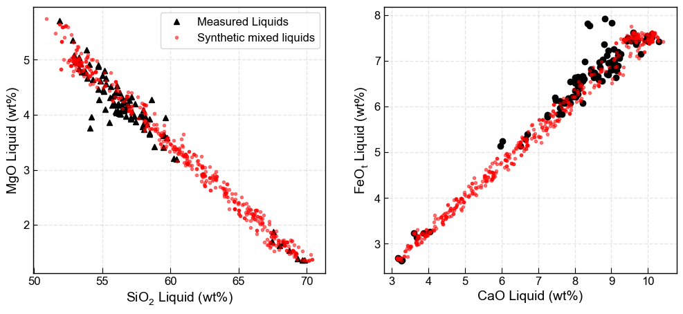
# Lets look at the naturally sampled liquids first
fig, ((ax1, ax2)) = plt.subplots(1, 2, figsize=(12, 5))
ax1.plot(myLiquids1['SiO2_Liq'], myLiquids1['MgO_Liq'], '^k', markerfacecolor='k', label='Measured Liquids')
ax2.plot(myLiquids1['CaO_Liq'], myLiquids1['FeOt_Liq'], 'ok', markerfacecolor='k', label='Measured Liquids')
[7]:
[<matplotlib.lines.Line2D at 0x184ffe2eb50>]
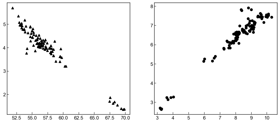
As Scruggs and Putrika (2018) showed, measured liquids have a clear Daly gap, and it is probably some cpxs crystallized from liquids between the analsed mafic and silicic end members
They use a mixing model to generate liquids lying between these two extremes to then feed into the Cpx-Liq spreadsheet (see https://www.youtube.com/watch?v=CjKvgXrah_k&list=PLnOXMT9X-AL_No_vUkkx8tYrahGQ1X4Kh&index=2&t=13s)
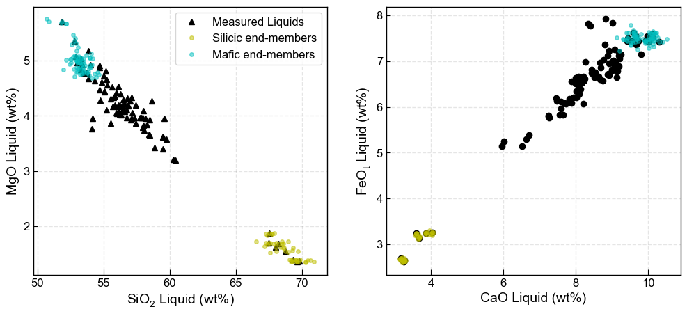
Here, we take liquids with SiO2_Liq>65 wt% (e.g., the evolved end member), add some noise to account for the silicic liquids we did not sample, in this case, 1% noise distributed normally, and make 5 synthetic samples per measured sample. This will be important if there are relatively large gaps between measured samples. We do the same to create a mafic end member, using a SiO2 and MgO filter
[8]:
Sil_endmember_noise1=pt.add_noise_sample_1phase(phase_comp=myLiquids1,  duplicates=5, filter_q='SiO2_Liq > 65',
                     phase_err_type="Perc", noise_percent=1, err_dist="normal", append=True)

Maf_endmember_noise1=pt.add_noise_sample_1phase(phase_comp=myLiquids1, duplicates=5,
                                                filter_q='SiO2_Liq < 53.8 & MgO_Liq>4',
                     phase_err_type="Perc", noise_percent=1, err_dist="normal", append=True)
All negative numbers replaced with zeros. If you wish to keep these, set positive=False
All negative numbers replaced with zeros. If you wish to keep these, set positive=False
We can plot these synthetic liquids, and see they cluster around measured liquid
[9]:
fig, ((ax1, ax2)) = plt.subplots(1, 2, figsize=(12, 5))
ax1.plot(myLiquids1['SiO2_Liq'], myLiquids1['MgO_Liq'], '^k', markerfacecolor='k', label='Measured Liquids')
ax1.plot(Sil_endmember_noise1['SiO2_Liq'], Sil_endmember_noise1['MgO_Liq'], 'oy',
         markeredgecolor='y', label='Silicic end-members',  markersize=4, alpha=0.5)
ax1.plot(Maf_endmember_noise1['SiO2_Liq'], Maf_endmember_noise1['MgO_Liq'], 'oc',
         markeredgecolor='c', label='Mafic end-members',  markersize=4, alpha=0.5)
ax1.set_xlabel('SiO$_2$ Liquid (wt%)')
ax1.set_ylabel('MgO Liquid (wt%)')
ax1.legend()
ax2.plot(myLiquids1['CaO_Liq'], myLiquids1['FeOt_Liq'], 'ok', markerfacecolor='k', label='Measured Liquids')
ax2.plot(Sil_endmember_noise1['CaO_Liq'], Sil_endmember_noise1['FeOt_Liq'], 'oy',
         markeredgecolor='y', label='Silicic end-members',  markersize=4, alpha=0.5)
ax2.plot(Maf_endmember_noise1['CaO_Liq'], Maf_endmember_noise1['FeOt_Liq'], 'oc',
         markeredgecolor='c', label='Mafic end-members',  markersize=4, alpha=0.5)
ax2.set_xlabel('CaO Liquid (wt%)')
ax2.set_ylabel('FeO$_t$ Liquid (wt%)')
ax1.grid(color = 'k', linestyle = '--', linewidth = 1, alpha = 0.1)
ax2.grid(color = 'k', linestyle = '--', linewidth = 1, alpha = 0.1)
fig.savefig('EndMembers.png', dpi=300, transparent=True)
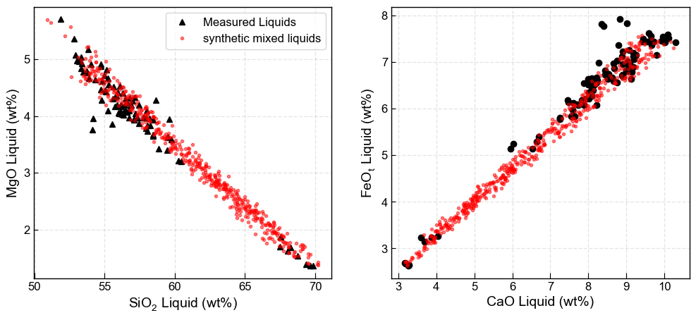
There are now a number of ways to mix these end-members to incorperate the liquid line of descent.
Option 1 - Mixing by bootstrapping, with no self mixing.
Takes end member 1 (Sil_endmember_noise1) and and end member 2 (Maf_endmember_noise1). Makes each input the length of the number of samples you specify with number samples. E.g., say when you generate your end member 1, you end up with 2000 samples. if you enter num_samples=500, it will randomly sample down to 500 samples. Conversely, if your end member only has 80 samples, it will scale it up by randomly resampling until you have 500 inputs.
Basically, if you generate more samples at the “end member” stage, they are generated with noise. If you generate more here, they are randomly sampled without adding noise.
The code then randomly mixes each element of end member 1 with end member 2 in a proportion determined by a random number generator between 0 and 1.
[10]:
# Make mixes
Mixed_noise5=pt.calculate_bootstrap_mixes(Sil_endmember_noise1, Maf_endmember_noise1,
                                          num_samples = 500, self_mixing = False)

# Plot them
fig, ((ax1, ax2)) = plt.subplots(1, 2, figsize=(12, 5))
ax1.plot(myLiquids1['SiO2_Liq'], myLiquids1['MgO_Liq'], '^k', label='Measured Liquids')
ax1.plot(Mixed_noise5['SiO2_Liq'], Mixed_noise5['MgO_Liq'], 'or', markerfacecolor='r',
         markersize=3, label='synthetic mixed liquids',  alpha=0.5)
ax1.set_xlabel('SiO$_2$ Liquid (wt%)')
ax1.set_ylabel('MgO Liquid (wt%)')
ax1.legend()
ax2.plot(myLiquids1['CaO_Liq'], myLiquids1['FeOt_Liq'], 'ok', label='Measured Liquids')
ax2.plot(Mixed_noise5['CaO_Liq'], Mixed_noise5['FeOt_Liq'], 'or', markerfacecolor='r',
         markersize=3,  alpha=0.5)

ax2.set_xlabel('CaO Liquid (wt%)')
ax2.set_ylabel('FeO$_t$ Liquid (wt%)')
ax1.grid(color = 'k', linestyle = '--', linewidth = 1, alpha = 0.1)
ax2.grid(color = 'k', linestyle = '--', linewidth = 1, alpha = 0.1)
Option 2 - Using self mixing
This will not only mix silicic and mafic end member, it will also mix between mafic end members, and between silic end-members.
This will cluster more liquids around where you have defined your end members, with more sparse coverage inbetween.
[11]:
Mixed_noise5_self=pt.calculate_bootstrap_mixes(Sil_endmember_noise1, Maf_endmember_noise1,
                                               num_samples = 500, self_mixing = True)

plt.plot(myLiquids1['SiO2_Liq'], myLiquids1['MgO_Liq'], 'ok', label='Measured Liquids')
plt.plot(Mixed_noise5_self['SiO2_Liq'], Mixed_noise5_self['MgO_Liq'], 'or', markerfacecolor='r',
         markersize=3,  alpha=0.5)
plt.xlabel('SiO$_2$ Liquid')
plt.ylabel('MgO Liquid')
[11]:
Text(0, 0.5, 'MgO Liquid')
If you want more even coverage in the middle, but some mixing at the edges, can use the keyword self_mixing=Partial
This will give half your liquids from self mixing, half from non-self mixing
[12]:
# Make mixes
Mixed_noise1_selfbig=pt.calculate_bootstrap_mixes(endmember1=Sil_endmember_noise1,
                                                  endmember2=Maf_endmember_noise1,
                                                  num_samples = 500, self_mixing = "Partial")


fig, ((ax1, ax2)) = plt.subplots(1, 2, figsize=(12, 5))

ax1.plot(myLiquids1['SiO2_Liq'], myLiquids1['MgO_Liq'], '^k', label='Measured Liquids')
ax1.plot(Mixed_noise1_selfbig['SiO2_Liq'], Mixed_noise1_selfbig['MgO_Liq'], 'or',
         markerfacecolor='r', markersize=3, label='Synthetic mixed liquids',  alpha=0.5)
ax1.set_xlabel('SiO$_2$ Liquid (wt%)')
ax1.set_ylabel('MgO Liquid (wt%)')
ax1.legend()
ax2.plot(myLiquids1['CaO_Liq'], myLiquids1['FeOt_Liq'], 'ok', label='Measured Liquids')
ax2.plot(Mixed_noise1_selfbig['CaO_Liq'], Mixed_noise1_selfbig['FeOt_Liq'], 'or',
         markerfacecolor='r', markersize=3,  alpha=0.5)

ax2.set_xlabel('CaO Liquid (wt%)')
ax2.set_ylabel('FeO$_t$ Liquid (wt%)')
ax1.grid(color = 'k', linestyle = '--', linewidth = 1, alpha = 0.1)
ax2.grid(color = 'k', linestyle = '--', linewidth = 1, alpha = 0.1)
fig.savefig('Mixing_EndMembers.svg', dpi=300)
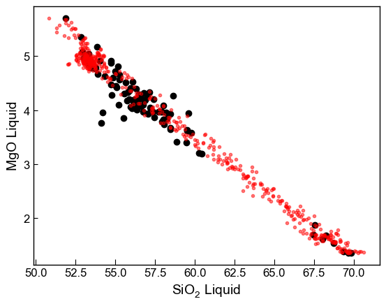
Now want to use these synthetic “partially-mixed” liquids for melt matching
First, lets combine these synthetic liquids with all measured liquids to get an even bigger dataset
[13]:
Liq_Comp=pd.concat([Mixed_noise1_selfbig.reset_index(drop=True),
                    myLiquids1.reset_index(drop=True)], axis=0).reset_index(drop=True).fillna(0)
Second, following Scruggs and Putirka (2018), lets allocate H2O as a function of SiO2 content in the melt
[14]:
Liq_Comp['H2O_Liq']=Liq_Comp['SiO2_Liq']*0.06995+0.383
Third, lets do melt matching
Uses fixed Kd of 0.27, +-0.03 following scruggs and Putirka
[15]:
melt_match_out_syn=pt.calculate_cpx_liq_press_temp_matching(liq_comps=Liq_Comp, cpx_comps=myCpxs1,
                                                    equationP="P_Neave2017", equationT="T_Put2008_eq33",
                                                    Kd_Match=0.27, Kd_Err=0.03)
Syn_Avs=melt_match_out_syn['Av_PTs']
Syn_All=melt_match_out_syn['All_PTs']
g:\my drive\postdoc\pymme\mybarometers\thermobar_outer\src\Thermobar\core.py:1561: FutureWarning: In a future version, the Index constructor will not infer numeric dtypes when passed object-dtype sequences (matching Series behavior)
  cpx_calc.loc[(AlVI_minus_Na<0), 'Jd']=cpx_calc['Al_VI_cat_6ox']
Considering N=286 Cpx & N=596 Liqs, which is a total of N=170456 Liq-Cpx pairs, be patient if this is >>1 million!
the code is evaluating Kd matches using Kd=0.27
32356 Matches remaining after initial Kd filter. Now moving onto iterative calculations
Finished calculating Ps and Ts, now just averaging the results. Almost there!
Done!!! I found a total of N=4925 Cpx-Liq matches using the specified filter. N=83 Cpx out of the N=286 Cpx that you input matched to 1 or more liquids
[16]:
Syn_Avs
[16]:
| Sample_ID_Cpx | # of Liqs Averaged | Mean_T_K_calc | Std_T_K_calc | Mean_P_kbar_calc | Std_P_kbar_calc | ID_CPX | Mean_Delta_T_K_Iter | Mean_Delta_P_kbar_Iter | Mean_Delta_Kd_Put2008 | Mean_Delta_Kd_Mas2013 | Mean_Delta_EnFs_Mollo13 | Mean_Delta_EnFs_Put1999 | Mean_Delta_CaTs_Put1999 | Mean_Delta_DiHd_Mollo13 | Mean_Delta_DiHd_Put1999 | Mean_Delta_CrCaTs_Put1999 | Mean_Delta_CaTi_Put1999 | Mean_DeltaKd_userselected=0.27 | Mean_SiO2_Liq | Mean_TiO2_Liq | Mean_Al2O3_Liq | Mean_FeOt_Liq | Mean_MnO_Liq | Mean_MgO_Liq | Mean_CaO_Liq | Mean_Na2O_Liq | Mean_K2O_Liq | Mean_Cr2O3_Liq | Mean_P2O5_Liq | Mean_H2O_Liq | Mean_Fe3Fet_Liq | Mean_NiO_Liq | Mean_CoO_Liq | Mean_CO2_Liq | Mean_SiO2_Liq_mol_frac | Mean_MgO_Liq_mol_frac | Mean_MnO_Liq_mol_frac | Mean_FeOt_Liq_mol_frac | Mean_CaO_Liq_mol_frac | Mean_Al2O3_Liq_mol_frac | Mean_Na2O_Liq_mol_frac | Mean_K2O_Liq_mol_frac | Mean_TiO2_Liq_mol_frac | Mean_P2O5_Liq_mol_frac | Mean_Cr2O3_Liq_mol_frac | Mean_Si_Liq_cat_frac | Mean_Mg_Liq_cat_frac | Mean_Mn_Liq_cat_frac | Mean_Fet_Liq_cat_frac | Mean_Ca_Liq_cat_frac | Mean_Al_Liq_cat_frac | Mean_Na_Liq_cat_frac | Mean_K_Liq_cat_frac | Mean_Ti_Liq_cat_frac | Mean_P_Liq_cat_frac | Mean_Cr_Liq_cat_frac | Mean_Mg_Number_Liq_NoFe3 | Mean_Mg_Number_Liq_Fe3 | Mean_ID_Liq | Mean_SiO2_Cpx | Mean_TiO2_Cpx | Mean_Al2O3_Cpx | Mean_FeOt_Cpx | Mean_MnO_Cpx | Mean_MgO_Cpx | Mean_CaO_Cpx | Mean_Na2O_Cpx | Mean_K2O_Cpx | Mean_Cr2O3_Cpx | Mean_Si_Cpx_cat_6ox | Mean_Mg_Cpx_cat_6ox | Mean_Fet_Cpx_cat_6ox | Mean_Ca_Cpx_cat_6ox | Mean_Al_Cpx_cat_6ox | Mean_Na_Cpx_cat_6ox | Mean_K_Cpx_cat_6ox | Mean_Mn_Cpx_cat_6ox | Mean_Ti_Cpx_cat_6ox | Mean_Cr_Cpx_cat_6ox | Mean_oxy_renorm_factor | Mean_Al_IV_cat_6ox | Mean_Al_VI_cat_6ox | Mean_En_Simple_MgFeCa_Cpx | Mean_Fs_Simple_MgFeCa_Cpx | Mean_Wo_Simple_MgFeCa_Cpx | Mean_Cation_Sum_Cpx | Mean_Ca_CaMgFe | Mean_Lindley_Fe3_Cpx | Mean_Lindley_Fe2_Cpx | Mean_Lindley_Fe3_Cpx_prop | Mean_CrCaTs | Mean_a_cpx_En | Mean_Mgno_Cpx | Mean_Jd | Mean_Jd_from 0=Na, 1=Al | Mean_CaTs | Mean_CaTi | Mean_DiHd_1996 | Mean_EnFs | Mean_DiHd_2003 | Mean_Di_Cpx | Mean_FeIII_Wang21 | Mean_FeII_Wang21 | Mean_Kd_Fe_Mg_Fe2 | Mean_Kd_Fe_Mg_Fe2_Lind | Mean_Kd_Fe_Mg_Fet | Mean_lnK_Jd_liq | Mean_lnK_Jd_DiHd_liq_1996 | Mean_lnK_Jd_DiHd_liq_2003 | Mean_Kd_Fe_Mg_IdealWB | Mean_Mgno_Liq_noFe3 | Mean_Mgno_Liq_Fe2 | Mean_DeltaFeMg_WB | Mean_T_Liq_MinP | Mean_T_Liq_MaxP | Mean_Kd_Ideal_Put | Mean_Kd_Ideal_Masotta | Mean_Delta_Kd_Put2008_I_M | Mean_DiHd_Pred_Put1999 | Mean_Delta_DiHd_I_M_Put1999 | Mean_DiHd_Pred_P2008 | Mean_Delta_DiHd_P2008 | Mean_DiHd_Pred_Mollo13 | Mean_Delta_DiHd_I_M_Mollo13 | Mean_EnFs_Pred_Put1999 | Mean_Delta_EnFs_I_M_Put1999 | Mean_EnFs_Pred_Mollo13 | Mean_Delta_EnFs_I_M_Mollo13 | Mean_CaTs_Pred_Put1999 | Mean_Delta_CaTs_I_M_Put1999 | Mean_CrCaTs_Pred_Put1999 | Mean_Delta_CrCaTs_I_M_Put1999 | Mean_CaTi_Pred_Put1999 | Mean_Delta_CaTi_I_M_Put1999 | Mean_Jd_Pred_Put1999 | Mean_Delta_Jd_Put1999 | Mean_Delta_Jd_I_M_Put1999 | Mean_DeltaKd_Kd_Match_userSp | Std_Delta_T_K_Iter | Std_Delta_P_kbar_Iter | Std_Delta_Kd_Put2008 | Std_Delta_Kd_Mas2013 | Std_Delta_EnFs_Mollo13 | Std_Delta_EnFs_Put1999 | Std_Delta_CaTs_Put1999 | Std_Delta_DiHd_Mollo13 | Std_Delta_DiHd_Put1999 | Std_Delta_CrCaTs_Put1999 | Std_Delta_CaTi_Put1999 | Std_DeltaKd_userselected=0.27 | Std_SiO2_Liq | Std_TiO2_Liq | Std_Al2O3_Liq | Std_FeOt_Liq | Std_MnO_Liq | Std_MgO_Liq | Std_CaO_Liq | Std_Na2O_Liq | Std_K2O_Liq | Std_Cr2O3_Liq | Std_P2O5_Liq | Std_H2O_Liq | Std_Fe3Fet_Liq | Std_NiO_Liq | Std_CoO_Liq | Std_CO2_Liq | Std_SiO2_Liq_mol_frac | Std_MgO_Liq_mol_frac | Std_MnO_Liq_mol_frac | Std_FeOt_Liq_mol_frac | Std_CaO_Liq_mol_frac | Std_Al2O3_Liq_mol_frac | Std_Na2O_Liq_mol_frac | Std_K2O_Liq_mol_frac | Std_TiO2_Liq_mol_frac | Std_P2O5_Liq_mol_frac | Std_Cr2O3_Liq_mol_frac | Std_Si_Liq_cat_frac | Std_Mg_Liq_cat_frac | Std_Mn_Liq_cat_frac | Std_Fet_Liq_cat_frac | Std_Ca_Liq_cat_frac | Std_Al_Liq_cat_frac | Std_Na_Liq_cat_frac | Std_K_Liq_cat_frac | Std_Ti_Liq_cat_frac | Std_P_Liq_cat_frac | Std_Cr_Liq_cat_frac | Std_Mg_Number_Liq_NoFe3 | Std_Mg_Number_Liq_Fe3 | Std_ID_Liq | Std_SiO2_Cpx | Std_TiO2_Cpx | Std_Al2O3_Cpx | Std_FeOt_Cpx | Std_MnO_Cpx | Std_MgO_Cpx | Std_CaO_Cpx | Std_Na2O_Cpx | Std_K2O_Cpx | Std_Cr2O3_Cpx | Std_Si_Cpx_cat_6ox | Std_Mg_Cpx_cat_6ox | Std_Fet_Cpx_cat_6ox | Std_Ca_Cpx_cat_6ox | Std_Al_Cpx_cat_6ox | Std_Na_Cpx_cat_6ox | Std_K_Cpx_cat_6ox | Std_Mn_Cpx_cat_6ox | Std_Ti_Cpx_cat_6ox | Std_Cr_Cpx_cat_6ox | Std_oxy_renorm_factor | Std_Al_IV_cat_6ox | Std_Al_VI_cat_6ox | Std_En_Simple_MgFeCa_Cpx | Std_Fs_Simple_MgFeCa_Cpx | Std_Wo_Simple_MgFeCa_Cpx | Std_Cation_Sum_Cpx | Std_Ca_CaMgFe | Std_Lindley_Fe3_Cpx | Std_Lindley_Fe2_Cpx | Std_Lindley_Fe3_Cpx_prop | Std_CrCaTs | Std_a_cpx_En | Std_Mgno_Cpx | Std_Jd | Std_Jd_from 0=Na, 1=Al | Std_CaTs | Std_CaTi | Std_DiHd_1996 | Std_EnFs | Std_DiHd_2003 | Std_Di_Cpx | Std_FeIII_Wang21 | Std_FeII_Wang21 | Std_Kd_Fe_Mg_Fe2 | Std_Kd_Fe_Mg_Fe2_Lind | Std_Kd_Fe_Mg_Fet | Std_lnK_Jd_liq | Std_lnK_Jd_DiHd_liq_1996 | Std_lnK_Jd_DiHd_liq_2003 | Std_Kd_Fe_Mg_IdealWB | Std_Mgno_Liq_noFe3 | Std_Mgno_Liq_Fe2 | Std_DeltaFeMg_WB | Std_T_Liq_MinP | Std_T_Liq_MaxP | Std_Kd_Ideal_Put | Std_Kd_Ideal_Masotta | Std_Delta_Kd_Put2008_I_M | Std_DiHd_Pred_Put1999 | Std_Delta_DiHd_I_M_Put1999 | Std_DiHd_Pred_P2008 | Std_Delta_DiHd_P2008 | Std_DiHd_Pred_Mollo13 | Std_Delta_DiHd_I_M_Mollo13 | Std_EnFs_Pred_Put1999 | Std_Delta_EnFs_I_M_Put1999 | Std_EnFs_Pred_Mollo13 | Std_Delta_EnFs_I_M_Mollo13 | Std_CaTs_Pred_Put1999 | Std_Delta_CaTs_I_M_Put1999 | Std_CrCaTs_Pred_Put1999 | Std_Delta_CrCaTs_I_M_Put1999 | Std_CaTi_Pred_Put1999 | Std_Delta_CaTi_I_M_Put1999 | Std_Jd_Pred_Put1999 | Std_Delta_Jd_Put1999 | Std_Delta_Jd_I_M_Put1999 | Std_DeltaKd_Kd_Match_userSp | |
|---|---|---|---|---|---|---|---|---|---|---|---|---|---|---|---|---|---|---|---|---|---|---|---|---|---|---|---|---|---|---|---|---|---|---|---|---|---|---|---|---|---|---|---|---|---|---|---|---|---|---|---|---|---|---|---|---|---|---|---|---|---|---|---|---|---|---|---|---|---|---|---|---|---|---|---|---|---|---|---|---|---|---|---|---|---|---|---|---|---|---|---|---|---|---|---|---|---|---|---|---|---|---|---|---|---|---|---|---|---|---|---|---|---|---|---|---|---|---|---|---|---|---|---|---|---|---|---|---|---|---|---|---|---|---|---|---|---|---|---|---|---|---|---|---|---|---|---|---|---|---|---|---|---|---|---|---|---|---|---|---|---|---|---|---|---|---|---|---|---|---|---|---|---|---|---|---|---|---|---|---|---|---|---|---|---|---|---|---|---|---|---|---|---|---|---|---|---|---|---|---|---|---|---|---|---|---|---|---|---|---|---|---|---|---|---|---|---|---|---|---|---|---|---|---|---|---|---|---|---|---|---|---|---|---|---|---|---|---|---|---|---|---|---|---|---|---|---|---|---|---|---|---|---|---|---|---|---|---|---|---|---|---|---|---|---|---|---|---|---|---|---|
| 0 | 12 | 107 | 1306.526526 | 9.376336 | -0.511727 | 0.452143 | 12 | 0.0 | 0.0 | 0.045284 | 0.145822 | 0.041715 | 0.043549 | 0.016400 | 0.037627 | 0.208505 | 0.001323 | 0.002261 | 0.016926 | 55.511476 | 0.677461 | 18.520169 | 6.906262 | 0.129007 | 4.425550 | 8.825517 | 3.068379 | 1.071846 | 0.0 | 0.095251 | 4.266028 | 0.0 | 0.0 | 0.0 | 0.0 | 0.599650 | 0.071272 | 0.001180 | 0.062393 | 0.102149 | 0.117898 | 0.032133 | 0.007384 | 0.005505 | 0.000436 | 0.0 | 0.517895 | 0.061557 | 0.001020 | 0.053889 | 0.088229 | 0.203649 | 0.055501 | 0.012754 | 0.004754 | 0.000752 | 0.0 | 0.532970 | 0.532970 | 389.401869 | 52.0030 | 0.3960 | 3.0110 | 7.3920 | 0.2120 | 16.5370 | 20.4390 | 0.1570 | 0.0 | 0.0910 | 1.913065 | 0.906915 | 0.227415 | 0.805627 | 0.130548 | 0.011198 | 0.0 | 0.006606 | 0.010958 | 0.002647 | 0.0 | 0.086935 | 0.043613 | 0.467492 | 0.117227 | 0.415281 | 4.014979 | 0.415281 | 0.029958 | 0.197457 | 0.131731 | 0.001323 | 0.169950 | 0.799511 | 0.011198 | 0.0 | 0.032415 | 0.027260 | 0.744629 | 0.194851 | 0.744629 | 0.591896 | 0.029958 | 0.197457 | 0.286340 | 0.248620 | 0.286340 | 1.308725 | -4.304148 | -4.304148 | 0.257709 | 0.532970 | 0.532970 | 0.028631 | 1264.189137 | 1464.092464 | 0.241056 | 0.140518 | -0.045284 | 0.953134 | 0.208505 | 0.779816 | 0.035186 | 0.782257 | 0.037627 | 0.151302 | -0.043549 | 0.153136 | -0.041715 | 0.016015 | -0.016400 | 0.0 | 0.001323 | 0.029411 | 0.002261 | 0.014203 | 0.003005 | 0.003005 | 0.016926 | 0.0 | 0.0 | 0.009054 | 0.012078 | 0.005501 | 0.003541 | 0.001094 | 0.015122 | 0.013988 | 0.0 | 0.001711 | 0.008420 | 1.405186 | 0.055049 | 0.349387 | 0.440793 | 0.007498 | 0.341567 | 0.551152 | 0.160972 | 0.222309 | 0.0 | 0.022173 | 0.098293 | 0.0 | 0.0 | 0.0 | 0.0 | 0.014673 | 0.005544 | 0.000069 | 0.004012 | 0.006379 | 0.002341 | 0.001680 | 0.001528 | 0.000447 | 0.000102 | 0.0 | 0.012447 | 0.004812 | 0.000060 | 0.003498 | 0.005600 | 0.004015 | 0.002830 | 0.002631 | 0.000382 | 0.000175 | 0.0 | 0.008377 | 0.008377 | 176.731908 | 0.0 | 0.0 | 0.0 | 0.0 | 0.0 | 0.0 | 0.0 | 0.0 | 0.0 | 0.0 | 0.0 | 0.0 | 0.0 | 0.0 | 0.0 | 0.0 | 0.0 | 0.0 | 0.0 | 0.0 | 0.0 | 0.0 | 0.0 | 0.0 | 0.0 | 0.0 | 0.0 | 0.0 | 0.0 | 0.0 | 0.0 | 0.0 | 0.0 | 0.0 | 0.0 | 0.0 | 0.0 | 0.0 | 0.0 | 0.0 | 0.0 | 0.0 | 0.0 | 0.0 | 0.009518 | 0.008264 | 0.009518 | 0.075789 | 0.157970 | 0.157970 | 0.0 | 0.008377 | 0.008377 | 0.009518 | 7.098376 | 9.519424 | 0.002276 | 0.005292 | 0.009054 | 0.013988 | 0.013988 | 0.010729 | 0.010729 | 0.015122 | 0.015122 | 0.003541 | 0.003541 | 0.005501 | 0.005501 | 0.001094 | 0.001094 | 0.0 | 0.0 | 0.001847 | 0.001711 | 0.000670 | 0.000670 | 0.000670 | 0.008420 |
| 1 | 16 | 68 | 1275.024984 | 18.731418 | 1.128074 | 0.762600 | 16 | 0.0 | 0.0 | 0.058895 | 0.150173 | 0.005556 | 0.010225 | 0.010407 | 0.034012 | 0.255719 | 0.000686 | 0.016809 | 0.024160 | 59.439491 | 0.605675 | 17.627905 | 5.809510 | 0.113055 | 3.474660 | 7.329222 | 3.417792 | 1.545027 | 0.0 | 0.097611 | 4.540792 | 0.0 | 0.0 | 0.0 | 0.0 | 0.641831 | 0.055928 | 0.001034 | 0.052460 | 0.084789 | 0.112170 | 0.035779 | 0.010643 | 0.004920 | 0.000446 | 0.0 | 0.553758 | 0.048257 | 0.000892 | 0.045264 | 0.073161 | 0.193556 | 0.061734 | 0.018363 | 0.004244 | 0.000770 | 0.0 | 0.516432 | 0.516432 | 353.176471 | 52.7020 | 0.2600 | 2.1400 | 7.1460 | 0.2480 | 14.6610 | 22.8580 | 0.3130 | 0.0 | 0.0470 | 1.946267 | 0.807137 | 0.220696 | 0.904454 | 0.093142 | 0.022411 | 0.0 | 0.007757 | 0.007222 | 0.001372 | 0.0 | 0.053733 | 0.039409 | 0.417711 | 0.114215 | 0.468074 | 4.010459 | 0.468074 | 0.020919 | 0.199777 | 0.094786 | 0.000686 | 0.068859 | 0.785275 | 0.022411 | 0.0 | 0.016998 | 0.018368 | 0.868403 | 0.079715 | 0.868403 | 0.676831 | 0.020919 | 0.199777 | 0.292225 | 0.264526 | 0.292225 | 1.815620 | -4.232141 | -4.232141 | 0.255061 | 0.516432 | 0.516432 | 0.037839 | 1227.897473 | 1415.661866 | 0.233330 | 0.142053 | -0.058895 | 1.124122 | 0.255719 | 0.792547 | 0.075855 | 0.881164 | 0.012761 | 0.069491 | -0.010225 | 0.083646 | 0.003930 | 0.006591 | -0.010407 | 0.0 | 0.000686 | 0.035177 | 0.016809 | 0.015487 | 0.006924 | 0.006924 | 0.024160 | 0.0 | 0.0 | 0.011989 | 0.008366 | 0.003237 | 0.001816 | 0.001115 | 0.016454 | 0.030607 | 0.0 | 0.005223 | 0.004156 | 2.582150 | 0.077450 | 0.639185 | 0.894890 | 0.013958 | 0.487720 | 1.057582 | 0.227751 | 0.331686 | 0.0 | 0.021648 | 0.180621 | 0.0 | 0.0 | 0.0 | 0.0 | 0.027867 | 0.007818 | 0.000127 | 0.008076 | 0.012186 | 0.004087 | 0.002408 | 0.002291 | 0.000632 | 0.000100 | 0.0 | 0.023922 | 0.006771 | 0.000110 | 0.006978 | 0.010562 | 0.006999 | 0.004072 | 0.003945 | 0.000543 | 0.000171 | 0.0 | 0.009543 | 0.009543 | 196.489257 | 0.0 | 0.0 | 0.0 | 0.0 | 0.0 | 0.0 | 0.0 | 0.0 | 0.0 | 0.0 | 0.0 | 0.0 | 0.0 | 0.0 | 0.0 | 0.0 | 0.0 | 0.0 | 0.0 | 0.0 | 0.0 | 0.0 | 0.0 | 0.0 | 0.0 | 0.0 | 0.0 | 0.0 | 0.0 | 0.0 | 0.0 | 0.0 | 0.0 | 0.0 | 0.0 | 0.0 | 0.0 | 0.0 | 0.0 | 0.0 | 0.0 | 0.0 | 0.0 | 0.0 | 0.010409 | 0.009422 | 0.010409 | 0.113965 | 0.310827 | 0.310827 | 0.0 | 0.009543 | 0.009543 | 0.007548 | 14.396057 | 19.145503 | 0.004614 | 0.004101 | 0.011989 | 0.030607 | 0.030607 | 0.019536 | 0.019536 | 0.035771 | 0.035771 | 0.001816 | 0.001816 | 0.005112 | 0.005112 | 0.001115 | 0.001115 | 0.0 | 0.0 | 0.005223 | 0.005223 | 0.000882 | 0.000882 | 0.000882 | 0.004156 |
| 2 | 26 | 5 | 1304.251537 | 4.271816 | 0.623434 | 0.441238 | 26 | 0.0 | 0.0 | 0.024975 | 0.131124 | 0.040744 | 0.031713 | 0.028638 | 0.033057 | 0.221923 | 0.000425 | 0.001505 | 0.016434 | 54.998000 | 0.796000 | 18.850000 | 7.664496 | 0.138000 | 3.948000 | 8.572000 | 3.258000 | 0.952000 | 0.0 | 0.110400 | 4.230110 | 0.0 | 0.0 | 0.0 | 0.0 | 0.597052 | 0.063890 | 0.001269 | 0.069589 | 0.099719 | 0.120601 | 0.034283 | 0.006590 | 0.006500 | 0.000507 | 0.0 | 0.513827 | 0.054986 | 0.001092 | 0.059886 | 0.085815 | 0.207572 | 0.059009 | 0.011345 | 0.005594 | 0.000873 | 0.0 | 0.478832 | 0.478832 | 546.200000 | 50.9350 | 0.4840 | 3.9410 | 8.0800 | 0.2120 | 15.7240 | 20.3010 | 0.1880 | 0.0 | 0.0290 | 1.887518 | 0.868653 | 0.250405 | 0.806056 | 0.172123 | 0.013508 | 0.0 | 0.006654 | 0.013491 | 0.000850 | 0.0 | 0.112482 | 0.059641 | 0.451222 | 0.130073 | 0.418706 | 4.019258 | 0.418706 | 0.038516 | 0.211888 | 0.153816 | 0.000425 | 0.163612 | 0.776230 | 0.013508 | 0.0 | 0.046133 | 0.033174 | 0.726324 | 0.196367 | 0.726324 | 0.560466 | 0.038516 | 0.211888 | 0.265483 | 0.224648 | 0.265483 | 1.431192 | -4.201248 | -4.201248 | 0.253379 | 0.478832 | 0.478832 | 0.015852 | 1257.214122 | 1454.738265 | 0.240508 | 0.134359 | -0.024975 | 0.948247 | 0.221923 | 0.748754 | 0.022430 | 0.759382 | 0.033057 | 0.164653 | -0.031713 | 0.155623 | -0.040744 | 0.017495 | -0.028638 | 0.0 | 0.000425 | 0.032574 | 0.001505 | 0.015204 | 0.001697 | 0.001697 | 0.016434 | 0.0 | 0.0 | 0.020773 | 0.014736 | 0.007091 | 0.006429 | 0.001232 | 0.015389 | 0.012336 | 0.0 | 0.001569 | 0.011433 | 0.819189 | 0.045056 | 0.501149 | 0.384837 | 0.004472 | 0.140428 | 0.327292 | 0.185391 | 0.221179 | 0.0 | 0.008933 | 0.057302 | 0.0 | 0.0 | 0.0 | 0.0 | 0.007203 | 0.002122 | 0.000042 | 0.003576 | 0.004117 | 0.003620 | 0.001821 | 0.001522 | 0.000368 | 0.000043 | 0.0 | 0.006664 | 0.001883 | 0.000036 | 0.003037 | 0.003458 | 0.005997 | 0.003170 | 0.002629 | 0.000316 | 0.000074 | 0.0 | 0.019329 | 0.019329 | 7.463243 | 0.0 | 0.0 | 0.0 | 0.0 | 0.0 | 0.0 | 0.0 | 0.0 | 0.0 | 0.0 | 0.0 | 0.0 | 0.0 | 0.0 | 0.0 | 0.0 | 0.0 | 0.0 | 0.0 | 0.0 | 0.0 | 0.0 | 0.0 | 0.0 | 0.0 | 0.0 | 0.0 | 0.0 | 0.0 | 0.0 | 0.0 | 0.0 | 0.0 | 0.0 | 0.0 | 0.0 | 0.0 | 0.0 | 0.0 | 0.0 | 0.0 | 0.0 | 0.0 | 0.0 | 0.021043 | 0.017806 | 0.021043 | 0.043221 | 0.062687 | 0.062687 | 0.0 | 0.019329 | 0.019329 | 0.017659 | 3.019301 | 4.041718 | 0.001039 | 0.007425 | 0.020773 | 0.012336 | 0.012336 | 0.014362 | 0.014362 | 0.015389 | 0.015389 | 0.006429 | 0.006429 | 0.007091 | 0.007091 | 0.001232 | 0.001232 | 0.0 | 0.0 | 0.002201 | 0.001569 | 0.000756 | 0.000756 | 0.000756 | 0.011433 |
| 3 | 29 | 175 | 1308.253432 | 12.493387 | -0.452758 | 0.517636 | 29 | 0.0 | 0.0 | 0.014170 | 0.117605 | 0.039377 | 0.044955 | 0.010736 | 0.021978 | 0.215655 | 0.002095 | 0.008902 | 0.017686 | 54.366620 | 0.680083 | 18.701915 | 7.119421 | 0.130635 | 4.779313 | 9.269542 | 2.969396 | 0.952359 | 0.0 | 0.091671 | 4.185945 | 0.0 | 0.0 | 0.0 | 0.0 | 0.587438 | 0.076996 | 0.001196 | 0.064340 | 0.107329 | 0.119087 | 0.031105 | 0.006563 | 0.005528 | 0.000419 | 0.0 | 0.507638 | 0.066544 | 0.001033 | 0.055604 | 0.092758 | 0.205825 | 0.053756 | 0.011341 | 0.004776 | 0.000725 | 0.0 | 0.544337 | 0.544337 | 322.965714 | 52.7470 | 0.3110 | 2.5050 | 6.4260 | 0.1780 | 16.8710 | 21.2650 | 0.1560 | 0.0 | 0.1450 | 1.927730 | 0.919174 | 0.196402 | 0.832697 | 0.107898 | 0.011054 | 0.0 | 0.005510 | 0.008549 | 0.004190 | 0.0 | 0.072270 | 0.035628 | 0.471789 | 0.100808 | 0.427403 | 4.013204 | 0.427403 | 0.026408 | 0.169994 | 0.134457 | 0.002095 | 0.146629 | 0.823941 | 0.011054 | 0.0 | 0.024574 | 0.023848 | 0.782180 | 0.166698 | 0.782180 | 0.641307 | 0.026408 | 0.169994 | 0.255587 | 0.221222 | 0.255587 | 1.357579 | -4.239749 | -4.239749 | 0.262253 | 0.544337 | 0.544337 | 0.012574 | 1265.536438 | 1465.907147 | 0.241471 | 0.137982 | -0.014117 | 0.997835 | 0.215655 | 0.804847 | 0.022693 | 0.803898 | 0.021718 | 0.121743 | -0.044955 | 0.127321 | -0.039377 | 0.013838 | -0.010736 | 0.0 | 0.002095 | 0.032750 | 0.008902 | 0.013823 | 0.002769 | 0.002769 | 0.017686 | 0.0 | 0.0 | 0.011287 | 0.013079 | 0.005935 | 0.003754 | 0.001088 | 0.018188 | 0.022174 | 0.0 | 0.002144 | 0.007304 | 1.700654 | 0.053445 | 0.364212 | 0.462570 | 0.008795 | 0.413862 | 0.692209 | 0.171776 | 0.217021 | 0.0 | 0.008898 | 0.118961 | 0.0 | 0.0 | 0.0 | 0.0 | 0.017426 | 0.006762 | 0.000082 | 0.004247 | 0.008125 | 0.002326 | 0.001782 | 0.001488 | 0.000432 | 0.000041 | 0.0 | 0.014648 | 0.005908 | 0.000071 | 0.003707 | 0.007119 | 0.004038 | 0.003009 | 0.002564 | 0.000370 | 0.000070 | 0.0 | 0.011833 | 0.011833 | 166.998173 | 0.0 | 0.0 | 0.0 | 0.0 | 0.0 | 0.0 | 0.0 | 0.0 | 0.0 | 0.0 | 0.0 | 0.0 | 0.0 | 0.0 | 0.0 | 0.0 | 0.0 | 0.0 | 0.0 | 0.0 | 0.0 | 0.0 | 0.0 | 0.0 | 0.0 | 0.0 | 0.0 | 0.0 | 0.0 | 0.0 | 0.0 | 0.0 | 0.0 | 0.0 | 0.0 | 0.0 | 0.0 | 0.0 | 0.0 | 0.0 | 0.0 | 0.0 | 0.0 | 0.0 | 0.012610 | 0.010915 | 0.012610 | 0.091352 | 0.187265 | 0.187265 | 0.0 | 0.011833 | 0.011833 | 0.006685 | 9.697536 | 13.009125 | 0.003033 | 0.005249 | 0.011354 | 0.022174 | 0.022174 | 0.012181 | 0.012132 | 0.018500 | 0.018500 | 0.003754 | 0.003754 | 0.005935 | 0.005935 | 0.001088 | 0.001088 | 0.0 | 0.0 | 0.002144 | 0.002144 | 0.000702 | 0.000702 | 0.000702 | 0.007304 |
| 4 | 30 | 11 | 1302.787795 | 7.103075 | -0.561921 | 0.219530 | 30 | 0.0 | 0.0 | 0.047838 | 0.146350 | 0.040597 | 0.036408 | 0.021698 | 0.050539 | 0.218011 | 0.000511 | 0.005276 | 0.024096 | 56.091818 | 0.691364 | 18.299545 | 7.020485 | 0.132273 | 4.064091 | 8.619545 | 3.165455 | 1.153636 | 0.0 | 0.088864 | 4.306623 | 0.0 | 0.0 | 0.0 | 0.0 | 0.606292 | 0.065489 | 0.001211 | 0.063464 | 0.099828 | 0.116564 | 0.033169 | 0.007955 | 0.005621 | 0.000407 | 0.0 | 0.523531 | 0.056551 | 0.001046 | 0.054798 | 0.086205 | 0.201298 | 0.057277 | 0.013739 | 0.004853 | 0.000702 | 0.0 | 0.508135 | 0.508135 | 558.000000 | 51.2810 | 0.5250 | 3.5980 | 8.0110 | 0.2110 | 16.1520 | 20.1810 | 0.1600 | 0.0 | 0.0350 | 1.893578 | 0.889123 | 0.247383 | 0.798441 | 0.156583 | 0.011455 | 0.0 | 0.006599 | 0.014582 | 0.001022 | 0.0 | 0.106422 | 0.050161 | 0.459508 | 0.127850 | 0.412642 | 4.018765 | 0.412642 | 0.037530 | 0.209853 | 0.151708 | 0.000511 | 0.174035 | 0.782325 | 0.011455 | 0.0 | 0.038706 | 0.033858 | 0.725366 | 0.205570 | 0.725366 | 0.564199 | 0.037530 | 0.209853 | 0.287988 | 0.244298 | 0.287988 | 1.289235 | -4.331453 | -4.331453 | 0.254512 | 0.508135 | 0.508135 | 0.035234 | 1260.920668 | 1459.707757 | 0.240150 | 0.141639 | -0.047838 | 0.943377 | 0.218011 | 0.770561 | 0.045196 | 0.775905 | 0.050539 | 0.169162 | -0.036408 | 0.164973 | -0.040597 | 0.017008 | -0.021698 | 0.0 | 0.000511 | 0.028582 | 0.005276 | 0.014609 | 0.003154 | 0.003154 | 0.024096 | 0.0 | 0.0 | 0.016767 | 0.012834 | 0.003715 | 0.005212 | 0.000616 | 0.007566 | 0.016315 | 0.0 | 0.002397 | 0.006181 | 0.718291 | 0.075898 | 0.231478 | 0.421157 | 0.005179 | 0.125754 | 0.320082 | 0.174477 | 0.131246 | 0.0 | 0.012466 | 0.050244 | 0.0 | 0.0 | 0.0 | 0.0 | 0.006722 | 0.002063 | 0.000046 | 0.003852 | 0.003747 | 0.001604 | 0.001816 | 0.000912 | 0.000619 | 0.000057 | 0.0 | 0.006162 | 0.001858 | 0.000039 | 0.003266 | 0.003354 | 0.002358 | 0.003027 | 0.001582 | 0.000527 | 0.000097 | 0.0 | 0.016407 | 0.016407 | 20.029978 | 0.0 | 0.0 | 0.0 | 0.0 | 0.0 | 0.0 | 0.0 | 0.0 | 0.0 | 0.0 | 0.0 | 0.0 | 0.0 | 0.0 | 0.0 | 0.0 | 0.0 | 0.0 | 0.0 | 0.0 | 0.0 | 0.0 | 0.0 | 0.0 | 0.0 | 0.0 | 0.0 | 0.0 | 0.0 | 0.0 | 0.0 | 0.0 | 0.0 | 0.0 | 0.0 | 0.0 | 0.0 | 0.0 | 0.0 | 0.0 | 0.0 | 0.0 | 0.0 | 0.0 | 0.017915 | 0.015197 | 0.017915 | 0.053479 | 0.095173 | 0.095173 | 0.0 | 0.016407 | 0.016407 | 0.013712 | 6.112737 | 8.191214 | 0.001727 | 0.006786 | 0.016767 | 0.016315 | 0.016315 | 0.006769 | 0.006769 | 0.007566 | 0.007566 | 0.005212 | 0.005212 | 0.003715 | 0.003715 | 0.000616 | 0.000616 | 0.0 | 0.0 | 0.002397 | 0.002397 | 0.000819 | 0.000819 | 0.000819 | 0.006181 |
| ... | ... | ... | ... | ... | ... | ... | ... | ... | ... | ... | ... | ... | ... | ... | ... | ... | ... | ... | ... | ... | ... | ... | ... | ... | ... | ... | ... | ... | ... | ... | ... | ... | ... | ... | ... | ... | ... | ... | ... | ... | ... | ... | ... | ... | ... | ... | ... | ... | ... | ... | ... | ... | ... | ... | ... | ... | ... | ... | ... | ... | ... | ... | ... | ... | ... | ... | ... | ... | ... | ... | ... | ... | ... | ... | ... | ... | ... | ... | ... | ... | ... | ... | ... | ... | ... | ... | ... | ... | ... | ... | ... | ... | ... | ... | ... | ... | ... | ... | ... | ... | ... | ... | ... | ... | ... | ... | ... | ... | ... | ... | ... | ... | ... | ... | ... | ... | ... | ... | ... | ... | ... | ... | ... | ... | ... | ... | ... | ... | ... | ... | ... | ... | ... | ... | ... | ... | ... | ... | ... | ... | ... | ... | ... | ... | ... | ... | ... | ... | ... | ... | ... | ... | ... | ... | ... | ... | ... | ... | ... | ... | ... | ... | ... | ... | ... | ... | ... | ... | ... | ... | ... | ... | ... | ... | ... | ... | ... | ... | ... | ... | ... | ... | ... | ... | ... | ... | ... | ... | ... | ... | ... | ... | ... | ... | ... | ... | ... | ... | ... | ... | ... | ... | ... | ... | ... | ... | ... | ... | ... | ... | ... | ... | ... | ... | ... | ... | ... | ... | ... | ... | ... | ... | ... | ... | ... | ... | ... | ... | ... | ... | ... | ... | ... | ... | ... | ... | ... | ... | ... | ... | ... | ... | ... | ... | ... | ... | ... | ... | ... | ... | ... | ... | ... | ... | ... | ... | ... | ... | ... | ... | ... | ... | ... | ... | ... | ... | ... | ... | ... | ... | ... |
| 78 | 262 | 148 | 1254.576384 | 17.851171 | -0.051798 | 0.316309 | 262 | 0.0 | 0.0 | 0.046197 | 0.124421 | 0.023658 | 0.102621 | 0.016496 | 0.023642 | 0.004637 | 0.000000 | 0.010735 | 0.012717 | 67.323874 | 0.443668 | 15.927379 | 3.355783 | 0.073223 | 1.858601 | 4.083106 | 4.056069 | 2.436763 | 0.0 | 0.108019 | 5.092305 | 0.0 | 0.0 | 0.0 | 0.0 | 0.727117 | 0.029925 | 0.000670 | 0.030311 | 0.047250 | 0.101372 | 0.042470 | 0.016788 | 0.003604 | 0.000494 | 0.0 | 0.626213 | 0.025775 | 0.000577 | 0.026107 | 0.040697 | 0.174610 | 0.073149 | 0.028916 | 0.003104 | 0.000851 | 0.0 | 0.495378 | 0.495378 | 253.587838 | 53.6456 | 0.4939 | 1.3572 | 9.6502 | 0.7088 | 19.3882 | 15.0159 | 0.2492 | 0.0 | 0.0000 | 1.958609 | 1.055260 | 0.294650 | 0.587406 | 0.058400 | 0.017640 | 0.0 | 0.021919 | 0.013564 | 0.000000 | 0.0 | 0.041391 | 0.017009 | 0.544702 | 0.152092 | 0.303206 | 4.007448 | 0.303206 | 0.014895 | 0.279754 | 0.050553 | 0.000000 | 0.379938 | 0.781721 | 0.017009 | 1.0 | 0.000000 | 0.020696 | 0.566710 | 0.391600 | 0.566710 | 0.435934 | 0.014895 | 0.279754 | 0.274456 | 0.260582 | 0.274456 | 1.224135 | -5.330586 | -5.330586 | 0.254400 | 0.495378 | 0.495378 | 0.020309 | 1213.639289 | 1396.749846 | 0.228260 | 0.150036 | -0.046197 | 0.568749 | 0.002039 | 0.536061 | 0.030649 | 0.590349 | 0.023639 | 0.288979 | -0.102621 | 0.367942 | -0.023658 | 0.016496 | 0.016496 | 0.0 | 0.000000 | 0.009961 | 0.010735 | 0.017653 | 0.000716 | 0.000716 | 0.012717 | 0.0 | 0.0 | 0.010914 | 0.012763 | 0.011958 | 0.020648 | 0.002521 | 0.012214 | 0.003570 | 0.0 | 0.001402 | 0.006917 | 1.617962 | 0.039107 | 0.344640 | 0.488002 | 0.007383 | 0.335629 | 0.648019 | 0.168129 | 0.173954 | 0.0 | 0.006298 | 0.113176 | 0.0 | 0.0 | 0.0 | 0.0 | 0.016827 | 0.005399 | 0.000068 | 0.004407 | 0.007492 | 0.002212 | 0.001789 | 0.001205 | 0.000319 | 0.000029 | 0.0 | 0.014225 | 0.004667 | 0.000059 | 0.003815 | 0.006481 | 0.003805 | 0.003000 | 0.002062 | 0.000275 | 0.000049 | 0.0 | 0.012609 | 0.012609 | 163.580596 | 0.0 | 0.0 | 0.0 | 0.0 | 0.0 | 0.0 | 0.0 | 0.0 | 0.0 | 0.0 | 0.0 | 0.0 | 0.0 | 0.0 | 0.0 | 0.0 | 0.0 | 0.0 | 0.0 | 0.0 | 0.0 | 0.0 | 0.0 | 0.0 | 0.0 | 0.0 | 0.0 | 0.0 | 0.0 | 0.0 | 0.0 | 0.0 | 0.0 | 0.0 | 0.0 | 0.0 | 0.0 | 0.0 | 0.0 | 0.0 | 0.0 | 0.0 | 0.0 | 0.0 | 0.013808 | 0.013110 | 0.013808 | 0.062740 | 0.335530 | 0.335530 | 0.0 | 0.012609 | 0.012609 | 0.013430 | 15.536983 | 20.582527 | 0.004448 | 0.003804 | 0.010914 | 0.005496 | 0.005496 | 0.005849 | 0.005849 | 0.012220 | 0.012220 | 0.020648 | 0.020648 | 0.011958 | 0.011958 | 0.002521 | 0.002521 | 0.0 | 0.0 | 0.001402 | 0.001402 | 0.000643 | 0.000561 | 0.000561 | 0.006917 |
| 79 | 263 | 292 | 1299.084968 | 21.851268 | 1.391518 | 0.842242 | 263 | 0.0 | 0.0 | 0.029937 | 0.123005 | 0.030792 | 0.046798 | 0.009402 | 0.030398 | 0.174693 | 0.000539 | 0.014554 | 0.009235 | 58.595322 | 0.609664 | 17.850118 | 5.951984 | 0.114667 | 3.790341 | 7.621043 | 3.332804 | 1.429863 | 0.0 | 0.098005 | 4.481743 | 0.0 | 0.0 | 0.0 | 0.0 | 0.632476 | 0.060981 | 0.001048 | 0.053719 | 0.088122 | 0.113534 | 0.034876 | 0.009847 | 0.004950 | 0.000448 | 0.0 | 0.545825 | 0.052637 | 0.000905 | 0.046369 | 0.076066 | 0.195972 | 0.060191 | 0.016992 | 0.004272 | 0.000773 | 0.0 | 0.531043 | 0.531043 | 326.414384 | 53.5085 | 0.3759 | 1.2288 | 6.8566 | 0.4798 | 16.1983 | 21.2414 | 0.3399 | 0.0 | 0.0371 | 1.967516 | 0.887919 | 0.210844 | 0.836858 | 0.053252 | 0.024232 | 0.0 | 0.014943 | 0.010397 | 0.001079 | 0.0 | 0.032484 | 0.020767 | 0.458726 | 0.108928 | 0.432346 | 4.007039 | 0.432346 | 0.014077 | 0.196766 | 0.066766 | 0.000539 | 0.133453 | 0.808103 | 0.020767 | 1.0 | 0.000000 | 0.016242 | 0.820076 | 0.139343 | 0.820076 | 0.653819 | 0.014077 | 0.196766 | 0.269159 | 0.251188 | 0.269159 | 1.782632 | -4.143602 | -4.143602 | 0.259307 | 0.531043 | 0.531043 | 0.011709 | 1249.058261 | 1443.874886 | 0.239222 | 0.146154 | -0.029937 | 0.994770 | 0.174693 | 0.757303 | 0.062773 | 0.819485 | -0.000592 | 0.092545 | -0.046798 | 0.108551 | -0.030792 | 0.009402 | 0.009402 | 0.0 | 0.000539 | 0.030796 | 0.014554 | 0.015165 | 0.005602 | 0.005602 | 0.009235 | 0.0 | 0.0 | 0.010678 | 0.012202 | 0.006893 | 0.002304 | 0.001584 | 0.017124 | 0.029787 | 0.0 | 0.003889 | 0.006777 | 2.682997 | 0.070315 | 0.617940 | 0.852000 | 0.014394 | 0.600830 | 1.144574 | 0.278197 | 0.328453 | 0.0 | 0.017280 | 0.187676 | 0.0 | 0.0 | 0.0 | 0.0 | 0.029352 | 0.009612 | 0.000131 | 0.007641 | 0.013131 | 0.003856 | 0.002944 | 0.002271 | 0.000568 | 0.000080 | 0.0 | 0.024821 | 0.008350 | 0.000113 | 0.006646 | 0.011431 | 0.006772 | 0.004981 | 0.003902 | 0.000491 | 0.000136 | 0.0 | 0.010482 | 0.010482 | 175.890301 | 0.0 | 0.0 | 0.0 | 0.0 | 0.0 | 0.0 | 0.0 | 0.0 | 0.0 | 0.0 | 0.0 | 0.0 | 0.0 | 0.0 | 0.0 | 0.0 | 0.0 | 0.0 | 0.0 | 0.0 | 0.0 | 0.0 | 0.0 | 0.0 | 0.0 | 0.0 | 0.0 | 0.0 | 0.0 | 0.0 | 0.0 | 0.0 | 0.0 | 0.0 | 0.0 | 0.0 | 0.0 | 0.0 | 0.0 | 0.0 | 0.0 | 0.0 | 0.0 | 0.0 | 0.011437 | 0.010673 | 0.011437 | 0.136576 | 0.348321 | 0.348321 | 0.0 | 0.010482 | 0.010482 | 0.009520 | 16.755540 | 22.385205 | 0.005326 | 0.003868 | 0.010678 | 0.029787 | 0.029787 | 0.020565 | 0.020565 | 0.034930 | 0.034930 | 0.002304 | 0.002304 | 0.006893 | 0.006893 | 0.001584 | 0.001584 | 0.0 | 0.0 | 0.003889 | 0.003889 | 0.001093 | 0.001093 | 0.001093 | 0.006777 |
| 80 | 264 | 77 | 1254.628230 | 12.761467 | 1.088352 | 0.251159 | 264 | 0.0 | 0.0 | 0.057212 | 0.133721 | 0.012134 | 0.100754 | 0.008233 | 0.043595 | 0.017704 | 0.000245 | 0.005145 | 0.015495 | 68.051867 | 0.427597 | 15.744021 | 3.136019 | 0.069794 | 1.668135 | 3.763169 | 4.100338 | 2.544967 | 0.0 | 0.108704 | 5.143228 | 0.0 | 0.0 | 0.0 | 0.0 | 0.735709 | 0.026889 | 0.000639 | 0.028357 | 0.043597 | 0.100307 | 0.042976 | 0.017550 | 0.003478 | 0.000497 | 0.0 | 0.633505 | 0.023154 | 0.000550 | 0.024419 | 0.037542 | 0.172744 | 0.074010 | 0.030224 | 0.002995 | 0.000857 | 0.0 | 0.486303 | 0.486303 | 265.467532 | 53.7403 | 0.2988 | 1.7901 | 9.8862 | 0.5881 | 18.3977 | 15.1352 | 0.3080 | 0.0 | 0.0169 | 1.968239 | 1.004500 | 0.302805 | 0.593935 | 0.077270 | 0.021871 | 0.0 | 0.018244 | 0.008232 | 0.000489 | 0.0 | 0.031761 | 0.045509 | 0.528339 | 0.159267 | 0.312394 | 3.995585 | 0.312394 | 0.000000 | 0.302805 | 0.000000 | 0.000245 | 0.365055 | 0.768369 | 0.021871 | 0.0 | 0.023638 | 0.004062 | 0.565991 | 0.370657 | 0.565991 | 0.428908 | -0.008829 | 0.311635 | 0.285495 | 0.285495 | 0.285495 | 1.450541 | -5.234625 | -5.234625 | 0.251917 | 0.486303 | 0.486303 | 0.033578 | 1209.187869 | 1390.837540 | 0.228283 | 0.151774 | -0.057212 | 0.583695 | 0.017704 | 0.537147 | 0.028845 | 0.609586 | 0.043595 | 0.269903 | -0.100754 | 0.358779 | -0.011878 | 0.015405 | -0.008233 | 0.0 | 0.000245 | 0.009207 | 0.005145 | 0.017796 | 0.004075 | 0.004075 | 0.015495 | 0.0 | 0.0 | 0.006970 | 0.007941 | 0.008775 | 0.015504 | 0.001720 | 0.009452 | 0.004757 | 0.0 | 0.001121 | 0.008166 | 1.236260 | 0.035515 | 0.241432 | 0.350544 | 0.005436 | 0.212091 | 0.440469 | 0.097325 | 0.111834 | 0.0 | 0.006853 | 0.086476 | 0.0 | 0.0 | 0.0 | 0.0 | 0.011720 | 0.003446 | 0.000051 | 0.003200 | 0.005149 | 0.001658 | 0.001032 | 0.000767 | 0.000294 | 0.000031 | 0.0 | 0.010054 | 0.002974 | 0.000044 | 0.002764 | 0.004445 | 0.002756 | 0.001719 | 0.001312 | 0.000253 | 0.000053 | 0.0 | 0.007126 | 0.007126 | 169.748311 | 0.0 | 0.0 | 0.0 | 0.0 | 0.0 | 0.0 | 0.0 | 0.0 | 0.0 | 0.0 | 0.0 | 0.0 | 0.0 | 0.0 | 0.0 | 0.0 | 0.0 | 0.0 | 0.0 | 0.0 | 0.0 | 0.0 | 0.0 | 0.0 | 0.0 | 0.0 | 0.0 | 0.0 | 0.0 | 0.0 | 0.0 | 0.0 | 0.0 | 0.0 | 0.0 | 0.0 | 0.0 | 0.0 | 0.0 | 0.0 | 0.0 | 0.0 | 0.0 | 0.0 | 0.008166 | 0.008166 | 0.008166 | 0.039495 | 0.235169 | 0.235169 | 0.0 | 0.007126 | 0.007126 | 0.008166 | 10.977486 | 14.537987 | 0.003174 | 0.002758 | 0.006970 | 0.004757 | 0.004757 | 0.003748 | 0.003748 | 0.009452 | 0.009452 | 0.015504 | 0.015504 | 0.009123 | 0.009123 | 0.001720 | 0.001720 | 0.0 | 0.0 | 0.001121 | 0.001121 | 0.000372 | 0.000372 | 0.000372 | 0.008166 |
| 81 | 265 | 42 | 1288.568145 | 11.909228 | 1.839449 | 0.303190 | 265 | 0.0 | 0.0 | 0.057237 | 0.139818 | 0.037054 | 0.065315 | 0.002504 | 0.038305 | 0.133610 | 0.000166 | 0.013731 | 0.023910 | 62.946554 | 0.520104 | 16.822650 | 4.678651 | 0.094889 | 2.783724 | 5.900643 | 3.671605 | 1.968996 | 0.0 | 0.100535 | 4.786111 | 0.0 | 0.0 | 0.0 | 0.0 | 0.679949 | 0.044831 | 0.000868 | 0.042268 | 0.068295 | 0.107087 | 0.038449 | 0.013567 | 0.004226 | 0.000460 | 0.0 | 0.586379 | 0.038664 | 0.000749 | 0.036454 | 0.058901 | 0.184703 | 0.066315 | 0.023399 | 0.003645 | 0.000793 | 0.0 | 0.514494 | 0.514494 | 228.571429 | 53.5292 | 0.3074 | 1.4979 | 8.0562 | 0.5608 | 16.2976 | 19.2569 | 0.3632 | 0.0 | 0.0114 | 1.974330 | 0.896110 | 0.248494 | 0.761007 | 0.065113 | 0.025973 | 0.0 | 0.017520 | 0.008528 | 0.000332 | 0.0 | 0.025670 | 0.039443 | 0.470248 | 0.130401 | 0.399351 | 3.997406 | 0.399351 | 0.000000 | 0.248494 | 0.000000 | 0.000166 | 0.203283 | 0.782894 | 0.025973 | 0.0 | 0.013470 | 0.006100 | 0.741270 | 0.201666 | 0.741270 | 0.571591 | -0.005188 | 0.253682 | 0.293910 | 0.293910 | 0.293910 | 1.820088 | -4.376905 | -4.376905 | 0.254618 | 0.514494 | 0.514494 | 0.039292 | 1237.567445 | 1428.512014 | 0.236673 | 0.154093 | -0.057237 | 0.874881 | 0.133610 | 0.693438 | 0.047832 | 0.779575 | 0.038305 | 0.136352 | -0.065315 | 0.164613 | -0.037054 | 0.010965 | -0.002504 | 0.0 | 0.000166 | 0.019832 | 0.013731 | 0.016349 | 0.009624 | 0.009624 | 0.023910 | 0.0 | 0.0 | 0.004079 | 0.005246 | 0.004588 | 0.004003 | 0.001024 | 0.014463 | 0.010148 | 0.0 | 0.001617 | 0.004893 | 1.286161 | 0.037167 | 0.260658 | 0.382211 | 0.006583 | 0.253942 | 0.535044 | 0.107583 | 0.148160 | 0.0 | 0.006349 | 0.089967 | 0.0 | 0.0 | 0.0 | 0.0 | 0.013157 | 0.004121 | 0.000061 | 0.003479 | 0.006199 | 0.001710 | 0.001128 | 0.001017 | 0.000307 | 0.000029 | 0.0 | 0.011051 | 0.003577 | 0.000053 | 0.003023 | 0.005386 | 0.002918 | 0.001885 | 0.001743 | 0.000264 | 0.000049 | 0.0 | 0.004196 | 0.004196 | 143.682941 | 0.0 | 0.0 | 0.0 | 0.0 | 0.0 | 0.0 | 0.0 | 0.0 | 0.0 | 0.0 | 0.0 | 0.0 | 0.0 | 0.0 | 0.0 | 0.0 | 0.0 | 0.0 | 0.0 | 0.0 | 0.0 | 0.0 | 0.0 | 0.0 | 0.0 | 0.0 | 0.0 | 0.0 | 0.0 | 0.0 | 0.0 | 0.0 | 0.0 | 0.0 | 0.0 | 0.0 | 0.0 | 0.0 | 0.0 | 0.0 | 0.0 | 0.0 | 0.0 | 0.0 | 0.004893 | 0.004893 | 0.004893 | 0.052413 | 0.192248 | 0.192248 | 0.0 | 0.004196 | 0.004196 | 0.004893 | 9.815143 | 13.078062 | 0.002917 | 0.002314 | 0.004079 | 0.010148 | 0.010148 | 0.007021 | 0.007021 | 0.014463 | 0.014463 | 0.004003 | 0.004003 | 0.004588 | 0.004588 | 0.001024 | 0.001024 | 0.0 | 0.0 | 0.001617 | 0.001617 | 0.000402 | 0.000402 | 0.000402 | 0.004893 |
| 82 | 277 | 238 | 1311.879993 | 17.478657 | 1.068502 | 0.748842 | 277 | 0.0 | 0.0 | 0.013330 | 0.114257 | 0.023908 | 0.031517 | 0.014283 | 0.024193 | 0.201697 | 0.003681 | 0.008181 | 0.017721 | 55.280861 | 0.659702 | 18.516711 | 6.862776 | 0.127302 | 4.573550 | 8.907121 | 3.046436 | 1.049028 | 0.0 | 0.094175 | 4.249896 | 0.0 | 0.0 | 0.0 | 0.0 | 0.597224 | 0.073669 | 0.001165 | 0.062011 | 0.103114 | 0.117890 | 0.031907 | 0.007228 | 0.005361 | 0.000431 | 0.0 | 0.515963 | 0.063655 | 0.001007 | 0.053579 | 0.089098 | 0.203707 | 0.055128 | 0.012487 | 0.004632 | 0.000744 | 0.0 | 0.542439 | 0.542439 | 321.768908 | 52.5100 | 0.3052 | 2.7442 | 6.2195 | 0.1422 | 16.2207 | 21.8581 | 0.2240 | 0.0 | 0.2542 | 1.923772 | 0.885910 | 0.190556 | 0.858020 | 0.118491 | 0.015911 | 0.0 | 0.004413 | 0.008411 | 0.007363 | 0.0 | 0.076228 | 0.042263 | 0.457956 | 0.098505 | 0.443539 | 4.012846 | 0.443539 | 0.025692 | 0.164864 | 0.134828 | 0.003681 | 0.117133 | 0.822975 | 0.015911 | 0.0 | 0.026352 | 0.024938 | 0.803048 | 0.136709 | 0.803048 | 0.658195 | 0.025692 | 0.164864 | 0.255329 | 0.220904 | 0.255329 | 1.676145 | -4.002887 | -4.002887 | 0.262073 | 0.542439 | 0.542439 | 0.012415 | 1262.308773 | 1461.591527 | 0.242340 | 0.141072 | -0.012989 | 1.004745 | 0.201697 | 0.775812 | 0.027701 | 0.807529 | 0.004481 | 0.105192 | -0.031517 | 0.112801 | -0.023908 | 0.012068 | -0.014283 | 0.0 | 0.003681 | 0.033119 | 0.008181 | 0.014114 | 0.001817 | 0.001817 | 0.017721 | 0.0 | 0.0 | 0.010975 | 0.012954 | 0.007082 | 0.003740 | 0.001409 | 0.014197 | 0.029653 | 0.0 | 0.002967 | 0.007678 | 2.310137 | 0.061413 | 0.482043 | 0.656520 | 0.011512 | 0.524574 | 0.954114 | 0.215354 | 0.268228 | 0.0 | 0.015216 | 0.161594 | 0.0 | 0.0 | 0.0 | 0.0 | 0.024305 | 0.008516 | 0.000106 | 0.005977 | 0.011109 | 0.003103 | 0.002244 | 0.001844 | 0.000499 | 0.000070 | 0.0 | 0.020559 | 0.007421 | 0.000092 | 0.005206 | 0.009692 | 0.005418 | 0.003805 | 0.003176 | 0.000429 | 0.000120 | 0.0 | 0.011838 | 0.011838 | 166.627003 | 0.0 | 0.0 | 0.0 | 0.0 | 0.0 | 0.0 | 0.0 | 0.0 | 0.0 | 0.0 | 0.0 | 0.0 | 0.0 | 0.0 | 0.0 | 0.0 | 0.0 | 0.0 | 0.0 | 0.0 | 0.0 | 0.0 | 0.0 | 0.0 | 0.0 | 0.0 | 0.0 | 0.0 | 0.0 | 0.0 | 0.0 | 0.0 | 0.0 | 0.0 | 0.0 | 0.0 | 0.0 | 0.0 | 0.0 | 0.0 | 0.0 | 0.0 | 0.0 | 0.0 | 0.012577 | 0.010881 | 0.012577 | 0.119852 | 0.258562 | 0.258562 | 0.0 | 0.011838 | 0.011838 | 0.007005 | 13.153599 | 17.626688 | 0.004237 | 0.004956 | 0.011378 | 0.029653 | 0.029653 | 0.016325 | 0.015521 | 0.027734 | 0.027734 | 0.003740 | 0.003740 | 0.007082 | 0.007082 | 0.001409 | 0.001409 | 0.0 | 0.0 | 0.002967 | 0.002967 | 0.000850 | 0.000807 | 0.000807 | 0.007678 |
83 rows × 271 columns
[17]:
Syn_Avs['Std_T_K_calc']
[17]:
0      9.376336
1     18.731418
2      4.271816
3     12.493387
4      7.103075
        ...
78    17.851171
79    21.851268
80    12.761467
81    11.909228
82    17.478657
Name: Std_T_K_calc, Length: 83, dtype: float64
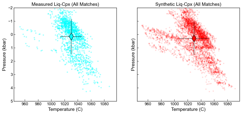
e.g., just using measured liquids, and using these synthetic liquids as well
[18]:
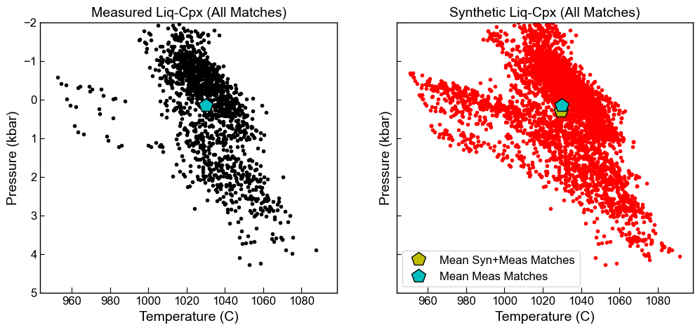
fig, ((ax1, ax2)) = plt.subplots(1, 2, figsize=(12, 5), sharex=True, sharey=True)

# Measured liquids only
ax1.set_title('Measured Liq-Cpx (All Matches)')
ax1.plot(Meas_All['T_K_calc']-273.15, Meas_All['P_kbar_calc'], '.k')
ax1.plot(np.nanmean(Meas_All['T_K_calc']-273.15), np.nanmean(Meas_All['P_kbar_calc']), 'pk',
        mfc='c', ms=15, label="Mean Meas Matches")

ax1.invert_yaxis()

ax1.set_xlabel('Temperature (C)')
ax1.set_ylabel('Pressure (kbar)')

# Synthetic liquids
ax2.set_title('Synthetic Liq-Cpx (All Matches)')
ax2.plot(Syn_All['T_K_calc']-273.15, Syn_All['P_kbar_calc'], '.r')

ax2.plot(np.nanmean(Syn_All['T_K_calc']-273.15), np.nanmean(Syn_All['P_kbar_calc']), 'pk',
        mfc='y', ms=15,label="Mean Syn+Meas Matches")
ax2.plot(np.nanmean(Meas_All['T_K_calc']-273.15), np.nanmean(Meas_All['P_kbar_calc']), 'pk',
        mfc='c', ms=15, label="Mean Meas Matches")

ax2.set_ylim([-2, 5])
ax2.invert_yaxis()
#ax2.set_xlim([700, 1200])

ax2.set_xlabel('Temperature (C)')
ax2.set_ylabel('Pressure (kbar)')
ax2.legend()
[18]:
<matplotlib.legend.Legend at 0x184804a46a0>
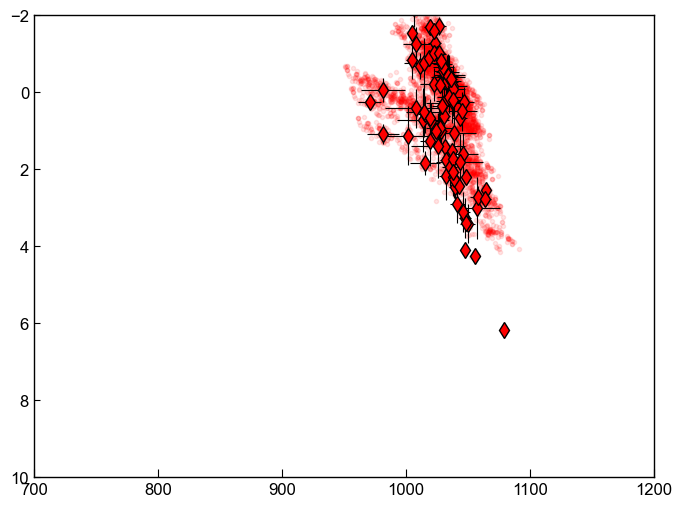
[19]:
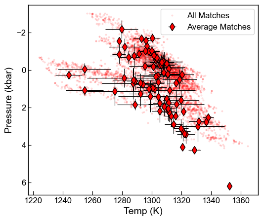
fig, (ax1) = plt.subplots(1, 1, figsize=(6, 5))
ax1.plot(Syn_All['T_K_calc'],  Syn_All['P_kbar_calc'], 'or',
         ms=2, mfc='red', alpha=0.1, label='All Matches')
ax1.errorbar(Syn_Avs['Mean_T_K_calc'],  Syn_Avs['Mean_P_kbar_calc'],
             xerr=Syn_Avs['Std_T_K_calc'].fillna(0),
             yerr=Syn_Avs['Std_P_kbar_calc'].fillna(0),
             fmt='d', ecolor='k', elinewidth=0.8,
              mfc='red', ms=8, mec='k', label='Average Matches')
ax1.invert_yaxis()
ax1.set_xlabel('Temp (K)')
ax1.set_ylabel('Pressure (kbar)')
ax1.legend()
fig.savefig('AllMatches_PT.png', dpi=300)
[20]:
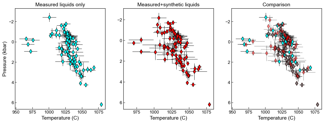
fig, ((ax1, ax2, ax3)) = plt.subplots(1, 3, figsize=(15, 5))#, sharex=True, sharey=True)
ax1.set_title('Measured liquids only')
ax1.errorbar(Meas_Avs['Mean_T_K_calc']-273.15,  Meas_Avs['Mean_P_kbar_calc'],
             xerr=Meas_Avs['Std_T_K_calc'], yerr=Meas_Avs['Std_P_kbar_calc'],
             fmt='d', ecolor='k', elinewidth=0.8, mfc='cyan', ms=8, mec='k', label='Pennys code')
ax1.invert_yaxis()

ax2.set_title('Measured+synthetic liquids')
ax2.errorbar(Syn_Avs['Mean_T_K_calc']-273.15,  Syn_Avs['Mean_P_kbar_calc'],
             xerr=Syn_Avs['Std_T_K_calc'], yerr=Syn_Avs['Std_P_kbar_calc'],
             fmt='d', ecolor='k', elinewidth=0.8, mfc='red', ms=8, mec='k', label='Pennys code')
ax2.invert_yaxis()

ax3.set_title('Comparison')
ax3.errorbar(Meas_Avs['Mean_T_K_calc']-273.15,  Meas_Avs['Mean_P_kbar_calc'],
             xerr=Meas_Avs['Std_T_K_calc'], yerr=Meas_Avs['Std_P_kbar_calc'],
             fmt='d', ecolor='k', elinewidth=0.8, mfc='cyan', ms=8, mec='k', label='Pennys code')
ax3.errorbar(Syn_Avs['Mean_T_K_calc']-273.15,  Syn_Avs['Mean_P_kbar_calc'],
             xerr=Syn_Avs['Std_T_K_calc'], yerr=Syn_Avs['Std_P_kbar_calc'],
             fmt='d', ecolor='k', elinewidth=0.8, mfc='red', ms=8, mec='k', label='Pennys code', alpha=0.5)
ax3.invert_yaxis()

ax1.set_xlabel('Temperature (C)')
ax2.set_xlabel('Temperature (C)')
ax3.set_xlabel('Temperature (C)')
ax1.set_ylabel('Pressure (kbar)')
[20]:
Text(0, 0.5, 'Pressure (kbar)')
Here, averaging all measurements
[21]:
fig, ((ax1, ax2)) = plt.subplots(1, 2, figsize=(12, 5), sharex=True, sharey=True)

ax1.set_title('Measured Liq-Cpx (All Matches)')
ax1.plot(Meas_All['T_K_calc']-273.15, Meas_All['P_kbar_calc'], '.', color='cyan', alpha=0.3)


ax1.errorbar(np.nanmean(Meas_All['T_K_calc']-273.15),  np.nanmean(Meas_All['P_kbar_calc']),
             xerr=np.nanstd(Meas_All['T_K_calc']-273.15), yerr=np.nanstd(Meas_All['P_kbar_calc']),
             fmt='d', ecolor='k', elinewidth=0.8, mfc='cyan', ms=15, mec='k', label='Pennys code', zorder=100)


#ax1.set_ylim([-2, 5])
ax1.invert_yaxis()

#ax1.set_xlim([700, 1200])
ax1.set_xlabel('Temperature (C)')
ax1.set_ylabel('Pressure (kbar)')
ax2.set_title('Synthetic Liq-Cpx (All Matches)')

ax2.plot(Syn_All['T_K_calc']-273.15, Syn_All['P_kbar_calc'], '.', color='red', alpha=0.1)
ax2.errorbar(np.nanmean(Syn_All['T_K_calc']-273.15),  np.nanmean(Syn_All['P_kbar_calc']),
             xerr=np.nanstd(Syn_All['T_K_calc']-273.15), yerr=np.nanstd(Syn_All['P_kbar_calc']),
             fmt='d', ecolor='k', elinewidth=0.8, mfc='red', ms=15, mec='k', label='Pennys code', zorder=100)


ax2.set_ylim([-2, 5])
ax2.invert_yaxis()
#ax2.set_xlim([700, 1200])

ax2.set_xlabel('Temperature (C)')
ax2.set_ylabel('Pressure (kbar)')
[21]:
Text(0, 0.5, 'Pressure (kbar)')
[22]:
#
fig, ((ax1)) = plt.subplots(1, figsize=(8, 6))

ax1.plot(Syn_All['T_K_calc']-273.15, Syn_All['P_kbar_calc'], '.', color='red', alpha=0.1)

ax1.errorbar(Syn_Avs['Mean_T_K_calc']-273.15,  Syn_Avs['Mean_P_kbar_calc'],
             xerr=Syn_Avs['Std_T_K_calc'], yerr=Syn_Avs['Std_P_kbar_calc'],
             fmt='d', ecolor='k', elinewidth=0.8, mfc='red', ms=8, mec='k', label='Pennys code')

ax1.set_xlim([700, 1200])
ax1.set_ylim([-2, 10])
ax1.invert_yaxis()

[ ]:
[ ]:
[ ]: