This page was generated from docs/Examples/Cpx_Cpx_Liq_Thermobarometry/Pyroxene_Ternary_Cpx_Example.ipynb. Interactive online version: .

Python Notebook Download

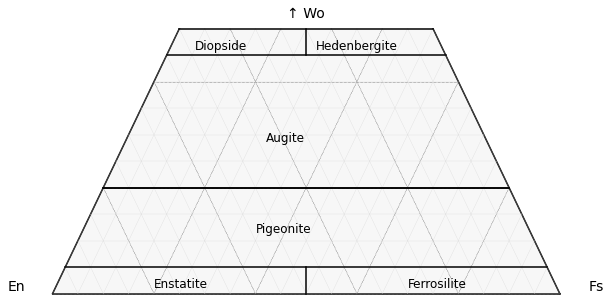
Pyroxene Classification Diagrams

• The function uses fields for the pyroxene ternary from Deer, Howie, and Zussman (1963).

• This function relies heavily on the ternary plot package from Marc Harper et al. 2015 - https://github.com/marcharper/python-ternary, if you use these figures, you must cite that (Marc Harper et al. (2015). python-ternary: Ternary Plots in Python. Zenodo. 10.5281/zenodo.594435) as well as Thermobar.

• You may have problems with this package if you have the separate “ternary” package installed (yes, there are python packages called ternary and python-ternary- Yay!). I (penny) got the error “module ternary has no attribute figure”, so had to uninstall the ternary I had through pip (pip uninstall ternary), and re-install python-ternary through conda in the command line “conda install python-ternary”. If you have everything in pip, or conda, keep in 1 environment, don’t follow my bad example here!

• You can download the excel spreadsheet with Cpx data from: https://github.com/PennyWieser/Thermobar/blob/main/docs/Examples/Cpx_Cpx_Liq_Thermobarometry/Cpx_Liq_Example.xlsx

# if you havent already done it, pip install Thermobar
#!pip install Thermobar

# pip install python-ternary
import ternary
#  We tested using ternary V.1.0.8
print(ternary.__version__)

import matplotlib.pyplot as plt
import numpy as np
import pandas as pd
import Thermobar as pt

Load in some Cpx compositions

out=pt.import_excel('Cpx_Liq_Example.xlsx', sheet_name="Sheet1")
my_input=out['my_input']
Liqs=out['Liqs']
Cpxs=out['Cpxs']

Lets transform these Cpx compositions into the 3 coordinates we need for plotting on our ternary diagrams.

• We are plotting in Mg-Fe-Ca space, so En is simply Mg/(Mg+Fet+Ca) etc.

cpx_comps_tern=pt.tern_points_px(px_comps=Cpxs)

Example 1

• Lets draw the diagram first to show you options

• (hold on, we’ll add data in a second)

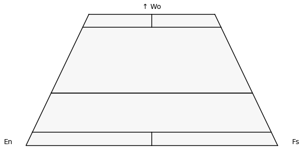
Example 1a - Simplicest, no grid, no labels, trimming off the top to make a quadrilateral

fig, tax = pt.plot_px_classification(figsize=(10, 5))

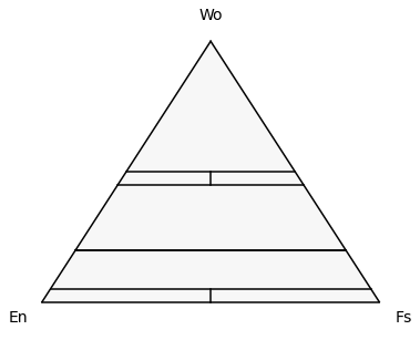
Example 1b - Lets keep the top!

fig, tax = pt.plot_px_classification(figsize=(6,5), cut_in_half=False)

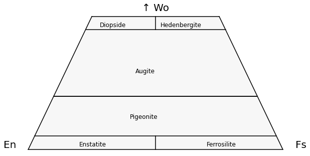
Example 1c- Lets add the field names on

• You can change font size using fontsize_component_labels to match the fig size

fig, tax = pt.plot_px_classification(figsize=(10, 5), labels=True,
                                     fontsize_component_labels=12,
                                    fontsize_axes_labels=20)

Example 1d - Lets add a grid

fig, tax = pt.plot_px_classification(figsize=(10, 5), labels=True, fontsize_component_labels=12,
                                     major_grid=True)

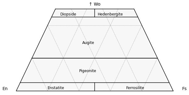
Example 1e - Lets add a minor grid

fig, tax = pt.plot_px_classification(figsize=(10, 5), labels=True, fontsize_component_labels=12,
                                     major_grid=True, minor_grid=True)

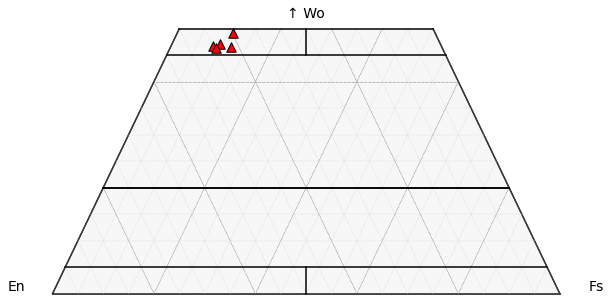
Example 2 - Lets add your data (simple to start!)

# First, define the plot as above.
fig, tax = pt.plot_px_classification(figsize=(10, 5),  fontsize_component_labels=12,
                                     major_grid=True, minor_grid=True)

## Now feed in your data we calculated at the start in terms of ternary axes!

tax.scatter(
    cpx_comps_tern,
    edgecolor="k",
    marker="^",
    facecolor="red",
    label='Label1',
   s=90
)

<AxesSubplot:>

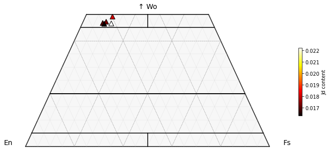
Example 3 - Lets color by Px Jd content

fig, tax = pt.plot_px_classification(figsize=(12, 5),  fontsize_component_labels=12,
                                     major_grid=True, minor_grid=True)

# We need to calculate Cpx compositions to get Jd
cpx_comps=pt.calculate_clinopyroxene_components(cpx_comps=Cpxs)
tax.scatter(
    cpx_comps_tern,
    c=cpx_comps["Jd"],
    vmin=np.min(cpx_comps["Jd"]),
    vmax=np.max(cpx_comps["Jd"]),
    s=100,
    edgecolor="k",
    marker="^",
    cmap="hot",
    colormap="hot",
    colorbar=True,
    cb_kwargs={"shrink": 0.5, "label": "Jd content"},

)
#  Uncomment to save the figure.
#fig.savefig('Pyroxene_Class.png', dpi=200)

<AxesSubplot:>