This page was generated from docs/Examples/Liquid_Ol_Liq_Themometry/Olivine_Liquid_thermometry.ipynb. Interactive online version: .

Olivine-Liquid thermometry

This script shows how to use the various options for olivine-liquid thermometry, including tests for equilibrium
It also shows how to calculate equilibrium olivine compositions from a measured liquid composition
we recomend you first got through the “Liquid_only thermometry.ipynb” example, as this demonstrates the various options for H2O and P which are also relevant here.
You can download the excel spreadsheet here for Liq-ol (paired up): https://github.com/PennyWieser/Thermobar/blob/main/docs/Examples/Liquid_Ol_Liq_Themometry/Liquid_only_Thermometry.xlsx
And the spreadsheet for individual Ol and Liquid here: https://github.com/PennyWieser/Thermobar/blob/main/docs/Examples/Liquid_Ol_Liq_Themometry/2018_Olivines_Glasses.xlsx

You need to install Thermobar once on your machine, if you haven’t done this yet, uncomment the line below (remove the #)

[1]:

#!pip install Thermobar

[2]:

# Loading various python things
import numpy as np
import pandas as pd
import matplotlib.pyplot as plt
import Thermobar as pt

[3]:

pt.__version__

[3]:

'1.0.12'

[4]:

# Setting plotting parameters
plt.rcParams["font.family"] = 'arial'
plt.rcParams["font.size"] =12
plt.rcParams["mathtext.default"] = "regular"
plt.rcParams["mathtext.fontset"] = "dejavusans"
plt.rcParams['patch.linewidth'] = 1
plt.rcParams['axes.linewidth'] = 1
plt.rcParams["xtick.direction"] = "in"
plt.rcParams["ytick.direction"] = "in"
plt.rcParams["ytick.direction"] = "in"
plt.rcParams["xtick.major.size"] = 6 # Sets length of ticks
plt.rcParams["ytick.major.size"] = 4 # Sets length of ticks
plt.rcParams["ytick.labelsize"] = 12 # Sets size of numbers on tick marks
plt.rcParams["xtick.labelsize"] = 12 # Sets size of numbers on tick marks
plt.rcParams["axes.titlesize"] = 14 # Overall title
plt.rcParams["axes.labelsize"] = 14 # Axes labels

Step 1 - load data

[5]:

out=pt.import_excel('Liquid_only_Thermometry.xlsx', sheet_name="Ol-Liq")
my_input=out['my_input']
myLiquids1=out['Liqs']
myOls1=out['Ols']
display(myOls1.head())
display(myLiquids1.head())

	SiO2_Ol	TiO2_Ol	Al2O3_Ol	FeOt_Ol	MnO_Ol	MgO_Ol	CaO_Ol	Cr2O3_Ol	Sample_ID_Ol
0	40.5	0.02	0.08	12.40	0.17	47.4	0.30	0.03	0
1	41.3	0.03	0.11	9.59	0.14	50.2	0.31	0.00	1
2	39.7	0.05	0.11	15.60	0.18	44.5	0.31	0.03	2
3	40.5	0.05	0.10	13.20	0.18	46.8	0.29	0.02	3
4	40.5	0.00	0.10	9.41	0.10	49.3	0.31	0.00	4

	SiO2_Liq	TiO2_Liq	Al2O3_Liq	FeOt_Liq	MnO_Liq	MgO_Liq	CaO_Liq	Na2O_Liq	K2O_Liq	Cr2O3_Liq	P2O5_Liq	H2O_Liq	Fe3Fet_Liq	Sample_ID_Liq
0	57.023602	0.623106	16.332899	4.36174	0.103851	4.19180	6.94858	3.59702	0.896895	0.000000	0.226584	5.59	0.2	0
1	57.658600	0.654150	17.194799	3.90621	0.084105	2.86892	5.91538	3.85948	1.018600	0.000000	0.214935	6.55	0.2	1
2	60.731201	0.862054	17.144199	4.07781	0.077488	2.50867	5.22075	4.45556	1.414160	0.000000	0.319638	3.14	0.2	2
3	61.532799	0.440860	16.508801	3.32990	0.037520	1.64150	4.34294	4.40860	1.407000	0.000000	0.215740	6.20	0.2	3
4	52.969101	0.803412	17.563000	5.93217	0.149472	3.78351	7.65110	3.80219	0.551178	0.037368	0.196182	6.58	0.2	4

Example 1 - Olivine-Liquid temperatures

It has been shown many times that olivines are not in equilirium with their co-erupted carrier melts. Thus, it is difficult to know what a meaningful Ol-Liq match is. Because of this, by default we return the value of Kd calculated for olivine-liquid as well as the calculated temperature in the “calculate_ol_liq_temp” function.
The function uses the Fe3Fet_Liq column in the user-entered spreadsheet, and calculates Fe/Mg in the liquid using only Fe2+ by default.
You can also specify a Fe3Fet_Liq ratio in the function itself (see later examples) to overwrite this value.
If the user doesn’t specify a column for Fe3Fet in the input, this value is set to zero.

1a - Putirka eq 22

[6]:

eq22_PHinput=pt.calculate_ol_liq_temp(liq_comps=myLiquids1, ol_comps=myOls1,  equationT="T_Put2008_eq22",
                                      P=my_input['P_kbar'])
eq22_PHinput

[6]:

	T_K_calc	Kd (Fe-Mg) Meas
0	1289.947705	0.314264
1	1229.813416	0.175383
2	1285.857491	0.269582
3	1198.240159	0.173799
4	1259.174284	0.152172
5	1244.931462	0.159554
6	1241.300118	0.215915
7	1199.601831	0.404699
8	1162.693468	0.314115
9	1339.466029	0.429135

1b - Specify eq_tests=True

FIf you specify eq_tests=True, the function also returns calculated Kd values for olivine-Liquid pairs so you can assess if olivine-liquids are in equilibrium.
A number of different equilibrium tests are returned, using Toplis, Matzen and Roeder and Emslie (preferred value=0.3 for Roeder and Emslie, 1970, =0.34 for Matzen, function of melt comp, temp and press for Toplis).
As before, here the Fe3Fet_Liq ratio in the spreadsheet is being used for calculations.

[7]:

eq22_PHinput=pt.calculate_ol_liq_temp(liq_comps=myLiquids1, ol_comps=myOls1,
                                      equationT="T_Put2008_eq22", P=my_input['P_kbar'], eq_tests=True)
eq22_PHinput

[7]:

	T_K_calc	Kd Meas	Kd calc (Toplis)	ΔKd, Toplis (M-P)	ΔKd, Roeder (M-P)	ΔKd, Matzen (M-P)	ΔKd, Shea (M-P)	SiO2_Liq	TiO2_Liq	Al2O3_Liq	...	Sample_ID_Ol	DMg_Meas	CNML	CSiO2L	NF	Den_Beat93
0	1289.947705	0.314264	0.325040	-0.010776	0.014264	-0.025736	-0.020736	57.023602	0.623106	16.332899	...	0	9.472619	0.170395	0.557471	-0.761843	9.819071
1	1229.813416	0.175383	0.308684	-0.133301	-0.124617	-0.164617	-0.159617	57.658600	0.654150	17.194799	...	1	14.186789	0.137941	0.570023	-0.816654	10.303635
2	1285.857491	0.269582	0.315891	-0.046309	-0.030418	-0.070418	-0.065418	60.731201	0.862054	17.144199	...	2	15.531216	0.122184	0.579288	-0.792785	10.250501
3	1198.240159	0.173799	0.296719	-0.122920	-0.126201	-0.166201	-0.161201	61.532799	0.440860	16.508801	...	3	23.753206	0.097626	0.605753	-0.767076	10.715090
4	1259.174284	0.152172	0.323766	-0.171594	-0.147828	-0.187828	-0.182828	52.969101	0.803412	17.563000	...	4	10.781292	0.186877	0.523030	-0.842157	10.215321
5	1244.931462	0.159554	0.324986	-0.165432	-0.140446	-0.180446	-0.175446	54.050201	0.857348	17.333300	...	5	12.276130	0.168070	0.533835	-0.833465	10.295063
6	1241.300118	0.215915	0.333878	-0.117963	-0.084085	-0.124085	-0.119085	55.656300	0.897984	17.117800	...	6	14.083460	0.145845	0.547483	-0.820914	10.324021
7	1199.601831	0.404699	0.391378	0.013321	0.104699	0.064699	0.069699	49.054699	0.488832	14.665000	...	7	7.372298	0.220053	0.554209	-0.789502	9.845140
8	1162.693468	0.314115	0.361834	-0.047718	0.014115	-0.025885	-0.020885	50.625099	0.334074	16.875000	...	8	10.509878	0.180293	0.551305	-0.873502	10.229233
9	1339.466029	0.429135	0.299720	0.129416	0.129135	0.089135	0.094135	51.403301	0.663880	18.019600	...	9	7.070601	0.228386	0.498172	-0.840523	9.673734

10 rows × 75 columns

If you want to access just the temperature from this panda dataframe, you do name[‘column heading’]
To get the output in Celcius, subtract -273.15

[8]:

Teq22_PHinput=eq22_PHinput['T_K_calc']-273.15 #converting temp to C
Teq22_PHinput

[8]:

0    1016.797705
1     956.663416
2    1012.707491
3     925.090159
4     986.024284
5     971.781462
6     968.150118
7     926.451831
8     889.543468
9    1066.316029
Name: T_K_calc, dtype: float64

Can also filter outputs, to only look at temps for pairs with delta K<=0.03 using the pandas loc function.
This basically says “give me the rows of eq22_PHinput where the column”ΔKd, Roeder” is less than or equal to 0.03 (e.g., in equilibrium)
Only 2 Ol-Liq pairs are in equilibrium here!

[9]:

T_in_eq=eq22_PHinput.loc[eq22_PHinput['ΔKd, Roeder (M-P)']<=0.03]
T_in_eq

[9]:

	T_K_calc	Kd Meas	Kd calc (Toplis)	ΔKd, Toplis (M-P)	ΔKd, Roeder (M-P)	ΔKd, Matzen (M-P)	ΔKd, Shea (M-P)	SiO2_Liq	TiO2_Liq	Al2O3_Liq	...	Sample_ID_Ol	DMg_Meas	CNML	CSiO2L	NF	Den_Beat93
0	1289.947705	0.314264	0.325040	-0.010776	0.014264	-0.025736	-0.020736	57.023602	0.623106	16.332899	...	0	9.472619	0.170395	0.557471	-0.761843	9.819071
1	1229.813416	0.175383	0.308684	-0.133301	-0.124617	-0.164617	-0.159617	57.658600	0.654150	17.194799	...	1	14.186789	0.137941	0.570023	-0.816654	10.303635
2	1285.857491	0.269582	0.315891	-0.046309	-0.030418	-0.070418	-0.065418	60.731201	0.862054	17.144199	...	2	15.531216	0.122184	0.579288	-0.792785	10.250501
3	1198.240159	0.173799	0.296719	-0.122920	-0.126201	-0.166201	-0.161201	61.532799	0.440860	16.508801	...	3	23.753206	0.097626	0.605753	-0.767076	10.715090
4	1259.174284	0.152172	0.323766	-0.171594	-0.147828	-0.187828	-0.182828	52.969101	0.803412	17.563000	...	4	10.781292	0.186877	0.523030	-0.842157	10.215321
5	1244.931462	0.159554	0.324986	-0.165432	-0.140446	-0.180446	-0.175446	54.050201	0.857348	17.333300	...	5	12.276130	0.168070	0.533835	-0.833465	10.295063
6	1241.300118	0.215915	0.333878	-0.117963	-0.084085	-0.124085	-0.119085	55.656300	0.897984	17.117800	...	6	14.083460	0.145845	0.547483	-0.820914	10.324021
8	1162.693468	0.314115	0.361834	-0.047718	0.014115	-0.025885	-0.020885	50.625099	0.334074	16.875000	...	8	10.509878	0.180293	0.551305	-0.873502	10.229233

8 rows × 75 columns

1c - You can also overwrite the spreadsheet Fe3Fet_Liq in the function itself

Here, we peform calculations using 30% Fe3+

[10]:

eq22_PHinput_30Fe3=pt.calculate_ol_liq_temp(liq_comps=myLiquids1, ol_comps=myOls1,
                                      equationT="T_Put2008_eq22", P=my_input['P_kbar'],
                                        Fe3Fet_Liq=0.3)
eq22_PHinput_30Fe3

[10]:

	T_K_calc	Kd (Fe-Mg) Meas
0	1289.947705	0.359158
1	1229.813416	0.200438
2	1285.857491	0.308094
3	1198.240159	0.198628
4	1259.174284	0.173911
5	1244.931462	0.182347
6	1241.300118	0.246761
7	1199.601831	0.462513
8	1162.693468	0.358989
9	1339.466029	0.490441

Example 2 - Considering all liquid-olivine matches

In reality, you have probably measured a load of glasses, and a load of olivines, but you dont know which ones match with which.
So, we have a matching algorithm, that returns all possible olivine-liquid pairs, which you can then filter.
Lets load the olivines and liquids separatly, as they will likely be different lenghts (and if you put them in one spreasdheet, you’ll end up with a load of NaNs which will cause issues!)

[11]:

# Loading in matrix glasses
out2018MG=pt.import_excel('2018_Olivines_Glasses.xlsx', sheet_name="LL4_MGs", suffix='_Liq')
my_input_MGs2018=out2018MG['my_input']
MGs2018=out2018MG['Liqs']

out2018Ols=pt.import_excel('2018_Olivines_Glasses.xlsx', sheet_name="LL4_Ols")
my_input_Ols2018=out2018Ols['my_input']
Ols2018=out2018Ols['Ols']

[12]:

display(MGs2018.head())
display(Ols2018.head())

	SiO2_Liq	TiO2_Liq	Al2O3_Liq	FeOt_Liq	MnO_Liq	MgO_Liq	CaO_Liq	Na2O_Liq	K2O_Liq	P2O5_Liq	Sample_ID_Liq
0	50.6243	2.8773	13.0360	11.8288	0.1830	5.8471	10.2471	2.5120	0.5234	0.2689	0
1	50.0975	2.8840	12.8885	11.2897	0.1769	5.8521	9.9658	2.4681	0.5305	0.2652	1
2	50.1346	2.8741	12.8953	11.8696	0.1814	5.8682	10.2012	2.4618	0.5778	0.2875	2
3	50.5233	2.8765	12.9818	11.3536	0.1454	5.8673	10.1806	2.6206	0.5206	0.2759	3
4	51.5840	2.9055	13.3290	11.5014	0.2286	5.8450	10.0408	2.1722	0.5565	0.2693	4

	SiO2_Ol	Al2O3_Ol	FeOt_Ol	MnO_Ol	MgO_Ol	CaO_Ol	NiO_Ol	Sample_ID_Ol
0	39.65300	0.04025	15.12365	0.20515	44.36500	0.25190	0.30635	0
1	39.79465	0.04405	12.84395	0.16570	45.94980	0.23245	0.37605	1
2	40.14520	0.04705	11.68440	0.14900	46.74595	0.23320	0.38705	2
3	39.53345	0.05060	16.92675	0.22125	43.10860	0.23345	0.26300	3
4	40.02325	0.05610	11.42200	0.15300	47.16475	0.22890	0.38110	4

[13]:

eq22_PHinput_30Fe3_Matching=pt.calculate_ol_liq_temp_matching(liq_comps=MGs2018,
                                        ol_comps=Ols2018,
                                      equationT="T_Put2008_eq22", P=5,
                                        Fe3Fet_Liq=0.3, eq_tests=True)
eq22_PHinput_30Fe3_Matching

Considering N=23 Ol & N=19 Liqs, which is a total of N=437 Liq-Ol pairs, be patient if this is >>1 million!

[13]:

	T_K_calc	Ol_Fo_Meas	Kd Meas	Kd calc (Toplis)	ΔKd, Toplis (M-P)	ΔKd, Roeder (M-P)	ΔKd, Matzen (M-P)	ΔKd, Shea (M-P)	SiO2_Liq	TiO2_Liq	...	Al_Ol_cat_frac	Na_Ol_cat_frac	K_Ol_cat_frac	Mn_Ol_cat_frac	Ti_Ol_cat_frac	DMg_Meas	CNML	CSiO2L	NF	Den_Beat93
0	1423.494959	0.839462	0.168506	0.287209	-0.118703	-0.131494	-0.171494	-0.166494	50.6243	2.87730	...	0.000399	0.0	0.0	0.001461	0.0	6.613445	0.286926	0.488362	-0.709158	9.825288
1	1427.581425	0.864445	0.176704	0.288398	-0.111695	-0.123296	-0.163296	-0.158296	50.0975	2.88400	...	0.000399	0.0	0.0	0.001461	0.0	6.510601	0.283867	0.490494	-0.713838	9.785899
2	1425.597182	0.877020	0.168533	0.287756	-0.119223	-0.131467	-0.171467	-0.166467	50.1346	2.87410	...	0.000399	0.0	0.0	0.001461	0.0	6.548023	0.288897	0.486713	-0.707200	9.810375
3	1426.830801	0.819485	0.176165	0.285916	-0.109751	-0.123835	-0.163835	-0.158835	50.5233	2.87650	...	0.000399	0.0	0.0	0.001461	0.0	6.563785	0.283546	0.489384	-0.709681	9.791213
4	1420.924109	0.880391	0.173241	0.294867	-0.121626	-0.126759	-0.166759	-0.161759	51.5840	2.90550	...	0.000399	0.0	0.0	0.001461	0.0	6.631816	0.281814	0.496419	-0.722465	9.840915
...	...	...	...	...	...	...	...	...	...	...	...	...	...	...	...	...	...	...	...	...	...
432	1447.022100	NaN	0.253368	0.297809	-0.044441	-0.046632	-0.086632	-0.081632	49.4837	2.87040	...	0.000443	0.0	0.0	0.001810	0.0	5.977917	0.289633	0.484568	-0.715446	9.632690
433	1446.896632	NaN	0.252072	0.297970	-0.045898	-0.047928	-0.087928	-0.082928	49.6879	2.88715	...	0.000443	0.0	0.0	0.001810	0.0	5.985175	0.289672	0.485115	-0.711773	9.633974
434	1441.532415	NaN	0.240536	0.296134	-0.055598	-0.059464	-0.099464	-0.094464	50.6177	2.82230	...	0.000443	0.0	0.0	0.001810	0.0	6.159819	0.285566	0.486791	-0.713133	9.671203
435	1445.556449	NaN	0.247346	0.298063	-0.050717	-0.052654	-0.092654	-0.087654	50.9821	2.81450	...	0.000443	0.0	0.0	0.001810	0.0	6.040965	0.286894	0.489008	-0.703872	9.641341
436	1443.554425	NaN	0.243931	0.297099	-0.053168	-0.056069	-0.096069	-0.091069	50.7999	2.81840	...	0.000443	0.0	0.0	0.001810	0.0	6.099735	0.286231	0.487901	-0.708494	9.656165

437 rows × 78 columns

Example 3 - Calculating equilibrium olivine Fo contents based on the liquid composition

3a - Roeder and Emslie, 1970

Here, using the Kd model of Roeder and Emslie, 1970, Kd=0.03+-0.03, for 20% Fe3
The function returns the Mg# of the liquid using Fe2+ based on the Fe3Fet ratio from the input spreadsheet, or specified by the user in the function (as in this example)
The Fet assumes that all Fe in the olivine and liquid is Fe2+
The Eq Fo contents are calculated using the Mg# with just Fe2, based on the Kd model shown in brackets

[12]:

Eq_Ol_Roeder=pt.calculate_eq_ol_content(liq_comps=myLiquids1, Kd_model="Roeder1970")
Eq_Ol_Roeder

[12]:

	Mg#_Liq_Fe2	Mg#_Liq_Fet	Eq Fo (Roeder, Kd=0.3)	Eq Fo (Roeder, Kd=0.33)	Eq Fo (Roeder, Kd=0.27)
0	0.681666	0.631416	0.877117	0.866470	0.888030
1	0.620707	0.566947	0.845080	0.832188	0.858378
2	0.578196	0.523041	0.820442	0.805970	0.835443
3	0.523445	0.467721	0.785468	0.768971	0.802688
4	0.586967	0.532031	0.825694	0.811549	0.840342
5	0.565465	0.510056	0.812653	0.797709	0.828169
6	0.528731	0.473003	0.789019	0.772716	0.806025
7	0.620033	0.566244	0.844705	0.831788	0.858030
8	0.583864	0.528846	0.823846	0.809585	0.838619
9	0.665729	0.614386	0.869086	0.857856	0.880615

[13]:

Eq_Ol_Roeder=pt.calculate_eq_ol_content(liq_comps=myLiquids1, Kd_model="Roeder1970", Fe3Fet_Liq=0.2)
Eq_Ol_Roeder

[13]:

	Mg#_Liq_Fe2	Mg#_Liq_Fet	Eq Fo (Roeder, Kd=0.3)	Eq Fo (Roeder, Kd=0.33)	Eq Fo (Roeder, Kd=0.27)
0	0.681666	0.631416	0.877117	0.866470	0.888030
1	0.620707	0.566947	0.845080	0.832188	0.858378
2	0.578196	0.523041	0.820442	0.805970	0.835443
3	0.523445	0.467721	0.785468	0.768971	0.802688
4	0.586967	0.532031	0.825694	0.811549	0.840342
5	0.565465	0.510056	0.812653	0.797709	0.828169
6	0.528731	0.473003	0.789019	0.772716	0.806025
7	0.620033	0.566244	0.844705	0.831788	0.858030
8	0.583864	0.528846	0.823846	0.809585	0.838619
9	0.665729	0.614386	0.869086	0.857856	0.880615

If you also specify the olivine compositions, it will add the measured Fo content as a column for comparison

[14]:

Eq_Ol_Roeder=pt.calculate_eq_ol_content(liq_comps=myLiquids1, ol_comps=myOls1,
                                     Kd_model="Roeder1970", Fe3Fet_Liq=0.2)
Eq_Ol_Roeder

[14]:

	Mg#_Liq_Fe2	Mg#_Liq_Fet	Eq Fo (Roeder, Kd=0.3)	Eq Fo (Roeder, Kd=0.33)	Eq Fo (Roeder, Kd=0.27)	Fo_meas
0	0.681666	0.631416	0.877117	0.866470	0.888030	0.872023
1	0.620707	0.566947	0.845080	0.832188	0.858378	0.903203
2	0.578196	0.523041	0.820442	0.805970	0.835443	0.835656
3	0.523445	0.467721	0.785468	0.768971	0.802688	0.863386
4	0.586967	0.532031	0.825694	0.811549	0.840342	0.903278
5	0.565465	0.510056	0.812653	0.797709	0.828169	0.890781
6	0.528731	0.473003	0.789019	0.772716	0.806025	0.838609
7	0.620033	0.566244	0.844705	0.831788	0.858030	0.801278
8	0.583864	0.528846	0.823846	0.809585	0.838619	0.817074
9	0.665729	0.614386	0.869086	0.857856	0.880615	0.822724

We can also specify to use the Kd model of Matzen (2011), where Kd=0.34 +-0.012

[15]:

Eq_Ol_Matzen=pt.calculate_eq_ol_content(liq_comps=myLiquids1,
                                        Kd_model="Matzen2011", Fe3Fet_Liq=0.2)
Eq_Ol_Matzen

[15]:

	Mg#_Liq_Fe2	Mg#_Liq_Fet	Eq Fo (Matzen, Kd=0.34)	Eq Fo (Matzen, Kd=0.352)	Eq Fo (Matzen, Kd=0.328)
0	0.681666	0.631416	0.862978	0.858825	0.867172
1	0.620707	0.566947	0.827977	0.822980	0.833035
2	0.578196	0.523041	0.801259	0.795678	0.806919
3	0.523445	0.467721	0.763625	0.757307	0.770049
4	0.586967	0.532031	0.806941	0.801479	0.812477
5	0.565465	0.510056	0.792848	0.787094	0.798688
6	0.528731	0.473003	0.767431	0.761182	0.773782
7	0.620033	0.566244	0.827569	0.822563	0.832637
8	0.583864	0.528846	0.804941	0.799437	0.810521
9	0.665729	0.614386	0.854176	0.849803	0.858595

3b - Toplis, 2005

This Kd expression is a bit more complicated, because the Toplis model is dependent on melt composition, as well as pressure, temperature, water content, and the olivine forsterite content
There are a number of options, firstly, you can specify a fixed olivine Fo content, P and T from input spreadsheet to perform calculations at

[16]:

Eq_Ol_Toplis_FixedFo=pt.calculate_eq_ol_content(liq_comps=myLiquids1, Kd_model="Toplis2005", Fe3Fet_Liq=0.2,
                     P=my_input['P_kbar'], T=my_input['Temperature_C']+273.15, ol_fo=0.8)
Eq_Ol_Toplis_FixedFo

[16]:

	Mg#_Liq_Fe2	Mg#_Liq_Fet	Kd (Toplis, input Fo)	Eq Fo (Toplis, input Fo)
0	0.681666	0.631416	0.343939	0.861610
1	0.620707	0.566947	0.354888	0.821787
2	0.578196	0.523041	0.339995	0.801262
3	0.523445	0.467721	0.343036	0.762017
4	0.586967	0.532031	0.373208	0.792006
5	0.565465	0.510056	0.372049	0.777663
6	0.528731	0.473003	0.365932	0.754055
7	0.620033	0.566244	0.451357	0.783331
8	0.583864	0.528846	0.434877	0.763388
9	0.665729	0.614386	0.336976	0.855286

Can do the same, but input olivine compositions, so the function uses the Fo content of each row to perform calculations (rather than a fixed Fo content).

[17]:

Eq_Ol_Toplis_FixedFo2=pt.calculate_eq_ol_content(liq_comps=myLiquids1, ol_comps=myOls1,
        Kd_model="Toplis2005", Fe3Fet_Liq=0.2, P=my_input['P_kbar'], T=my_input['Temperature_C'])
Eq_Ol_Toplis_FixedFo2

[17]:

	Mg#_Liq_Fe2	Mg#_Liq_Fet	Kd (Toplis, input Fo)	Eq Fo (Toplis, input Fo)	Fo_meas
0	0.681666	0.631416	0.262240	0.890897	0.872023
1	0.620707	0.566947	0.270643	0.858089	0.903203
2	0.578196	0.523041	0.276728	0.832031	0.835656
3	0.523445	0.467721	0.274170	0.800249	0.863386
4	0.586967	0.532031	0.290580	0.830239	0.903278
5	0.565465	0.510056	0.292062	0.816702	0.890781
6	0.528731	0.473003	0.297262	0.790541	0.838609
7	0.620033	0.566244	0.375747	0.812833	0.801278
8	0.583864	0.528846	0.358296	0.796579	0.817074
9	0.665729	0.614386	0.276607	0.878049	0.822724

However, this is clearly a bit of a backwards arguement if olivines and liquids aren’t in equilibrium, because that Fo content isn’t relevant, and you are having to use a Fo content to calculate a Fo content…
Instead, if you don’t specify Fo or an olivine content, the function will iterate Kd and olivine Fo content, starting from an olivine Fo content of 0.95 to reach an olivine content in equilibrium with your liquid for the toplis model

[18]:

Eq_Ol_Toplis_IterFo=pt.calculate_eq_ol_content(liq_comps=myLiquids1, Kd_model="Toplis2005", Fe3Fet_Liq=0.2,
                                                P=10, T=my_input['Temperature_C']+273.15)
Eq_Ol_Toplis_IterFo

[18]:

	Mg#_Liq_Fe2	Mg#_Liq_Fet	Kd (Toplis, Iter)	Eq Fo (Toplis, Iter)
0	0.681666	0.631416	0.340829	0.862690
1	0.620707	0.566947	0.358919	0.820127
2	0.578196	0.523041	0.345482	0.798700
3	0.523445	0.467721	0.356696	0.754863
4	0.586967	0.532031	0.381278	0.788460
5	0.565465	0.510056	0.383301	0.772469
6	0.528731	0.473003	0.382311	0.745844
7	0.620033	0.566244	0.463462	0.778805
8	0.583864	0.528846	0.451827	0.756413
9	0.665729	0.614386	0.332066	0.857093

You might not know temperature, which is needed for Toplis.
But, you have olivine-only thermometers at your fingertips, which can be input into the Eq ol content function.
Here we use one of the adapted olivine-liquid thermometers which use calulated DMg from the liquid rather than measured DMg.

[19]:

T_Calc_22=pt.calculate_liq_only_temp(liq_comps=myLiquids1, equationT="T_Put2008_eq22_BeattDMg",
                                     P=my_input['P_kbar'])

Eq_Ol_Toplis_IterFo_calcT=pt.calculate_eq_ol_content(liq_comps=myLiquids1, Kd_model="Toplis2005",
                          Fe3Fet_Liq=0.2, P=my_input['P_kbar'], T=T_Calc_22)

Eq_Ol_Toplis_IterFo_calcT

[19]:

	Mg#_Liq_Fe2	Mg#_Liq_Fet	Kd (Toplis, Iter)	Eq Fo (Toplis, Iter)
0	0.681666	0.631416	0.336288	0.864271
1	0.620707	0.566947	0.332721	0.831037
2	0.578196	0.523041	0.324101	0.808775
3	0.523445	0.467721	0.317484	0.775769
4	0.586967	0.532031	0.354413	0.800390
5	0.565465	0.510056	0.353012	0.786612
6	0.528731	0.473003	0.349961	0.762237
7	0.620033	0.566244	0.404831	0.801226
8	0.583864	0.528846	0.385667	0.784390
9	0.665729	0.614386	0.319173	0.861875

3c - Putirka (2016)

Equations 8a-8c are for when the proportion of Fe3 is known
Equations 9a-c are for when Fe is entered as Fet
Equation 8b and 9b require pressure, so if a presure isn’t entered, you dont get these outputs
Similarly, equation 9b requires an estimate of fo2

[20]:

## Here, we dont specify fo2 or P, so only get 8a, 8c, 9a +- errors back
Eq_Ol_Put_noP_fo2=pt.calculate_eq_ol_content(liq_comps=myLiquids1, Kd_model="Putirka2016",
                  Fe3Fet_Liq=0.2)
Eq_Ol_Put_noP_fo2.head()

g:\my drive\postdoc\pymme\mybarometers\thermobar_outer\src\Thermobar\mineral_equilibrium.py:214: UserWarning: Putirka (2016) Kd models equation 8b and 9b are P-dependent you need to enter a P in kbar to get these outputs
  w.warn(

[20]:

	Mg#_Liq_Fe2	Mg#_Liq_Fet	Eq Fo (Putirka 8a Fe2, Kd=0.33)	Eq Fo (Putirka 8a Fe2, Kd=0.33-0.044)	Eq Fo (Putirka 8a Fe2, Kd=0.33+0.044)	Calc Kd (Putirka 8c, Fe2)	Eq Fo (Putirka 8c Fe2)	Eq Fo (Putirka 9a Fet, Kd=0.29)	Eq Fo (Putirka 9a Fet, Kd=0.29-0.051)	Eq Fo (Putirka 9a Fet, Kd=0.29+0.051)
0	0.681666	0.631416	0.866470	0.882176	0.851313	0.346039	0.860883	0.855223	0.877567	0.877567
1	0.620707	0.566947	0.832188	0.851234	0.813975	0.346004	0.825469	0.818658	0.845626	0.845626
2	0.578196	0.523041	0.805970	0.827375	0.785645	0.348050	0.797507	0.790858	0.821056	0.821056
3	0.523445	0.467721	0.768971	0.793411	0.745992	0.349700	0.758510	0.751864	0.786171	0.786171
4	0.586967	0.532031	0.811549	0.832466	0.791657	0.339147	0.807332	0.796761	0.826295	0.826295

[21]:

## Here, we specify fo2 andd P, so only get 8b and 9b outputs as well.
Eq_Ol_Put_P_fo2=pt.calculate_eq_ol_content(liq_comps=myLiquids1, Kd_model="Putirka2016",
                                           Fe3Fet_Liq=0.2, logfo2=-10, P=5)
Eq_Ol_Put_P_fo2.head()

[21]:

	Mg#_Liq_Fe2	Mg#_Liq_Fet	Eq Fo (Putirka 8a Fe2, Kd=0.33)	Eq Fo (Putirka 8a Fe2, Kd=0.33-0.044)	Eq Fo (Putirka 8a Fe2, Kd=0.33+0.044)	Calc Kd (Putirka 8c, Fe2)	Eq Fo (Putirka 8c Fe2)	Eq Fo (Putirka 9a Fet, Kd=0.29)	Eq Fo (Putirka 9a Fet, Kd=0.29-0.051)	Eq Fo (Putirka 9a Fet, Kd=0.29+0.051)	Calc Kd (Putirka 8b, Fe2)	Eq Fo (Putirka 8b Fe2)	Calc Kd (Putirka 9b, Fet)	Eq Fo (Putirka 9b Fet)
0	0.681666	0.631416	0.866470	0.882176	0.851313	0.346039	0.860883	0.855223	0.877567	0.877567	0.349228	0.859781	0.308935	0.873919
1	0.620707	0.566947	0.832188	0.851234	0.813975	0.346004	0.825469	0.818658	0.845626	0.845626	0.349509	0.824013	0.307039	0.842019
2	0.578196	0.523041	0.805970	0.827375	0.785645	0.348050	0.797507	0.790858	0.821056	0.821056	0.353321	0.795068	0.305758	0.817624
3	0.523445	0.467721	0.768971	0.793411	0.745992	0.349700	0.758510	0.751864	0.786171	0.786171	0.355555	0.755456	0.308271	0.780850
4	0.586967	0.532031	0.811549	0.832466	0.791657	0.339147	0.807332	0.796761	0.826295	0.826295	0.339543	0.807150	0.299996	0.825696

3d - All Models

We can also specify Kd_model=“All” to get results from all of these models
Here we are using the temperature from the adapted ol-liq thermometer applied to just liquid compositions

[22]:

Eq_Ol_IterFo_calcT=pt.calculate_eq_ol_content(liq_comps=myLiquids1, Kd_model="All", Fe3Fet_Liq=0.2,
                                                P=my_input['P_kbar'], T=T_Calc_22)
Eq_Ol_IterFo_calcT

[22]:

	Mg#_Liq_Fe2	Mg#_Liq_Fet	Eq Fo (Shea, Kd=0.335)	Eq Fo (Shea, Kd=0.325)	Eq Fo (Shea, Kd=0.345)	Eq Fo (Roeder, Kd=0.3)	Eq Fo (Roeder, Kd=0.33)	Eq Fo (Roeder, Kd=0.27)	Eq Fo (Matzen, Kd=0.34)	Eq Fo (Matzen, Kd=0.352)	...	Eq Fo (Putirka 8a Fe2, Kd=0.33)	Eq Fo (Putirka 8a Fe2, Kd=0.33-0.044)	Eq Fo (Putirka 8a Fe2, Kd=0.33+0.044)	Calc Kd (Putirka 8c, Fe2)	Eq Fo (Putirka 8c Fe2)	Eq Fo (Putirka 9a Fet, Kd=0.29)	Eq Fo (Putirka 9a Fet, Kd=0.29-0.051)	Eq Fo (Putirka 9a Fet, Kd=0.29+0.051)	Calc Kd (Putirka 8b, Fe2)	Eq Fo (Putirka 8b Fe2)
0	0.681666	0.631416	0.864721	0.861243	0.868227	0.877117	0.866470	0.888030	0.862978	0.858825	...	0.866470	0.882176	0.851313	0.346039	0.860883	0.855223	0.877567	0.877567	0.346828	0.860610
1	0.620707	0.566947	0.830077	0.825888	0.834309	0.845080	0.832188	0.858378	0.827977	0.822980	...	0.832188	0.851234	0.813975	0.346004	0.825469	0.818658	0.845626	0.845626	0.347909	0.824677
2	0.578196	0.523041	0.803608	0.798924	0.808347	0.820442	0.805970	0.835443	0.801259	0.795678	...	0.805970	0.827375	0.785645	0.348050	0.797507	0.790858	0.821056	0.821056	0.353321	0.795068
3	0.523445	0.467721	0.766289	0.760980	0.771672	0.785468	0.768971	0.802688	0.763625	0.757307	...	0.768971	0.793411	0.745992	0.349700	0.758510	0.751864	0.786171	0.786171	0.355555	0.755456
4	0.586967	0.532031	0.809238	0.804656	0.813873	0.825694	0.811549	0.840342	0.806941	0.801479	...	0.811549	0.832466	0.791657	0.339147	0.807332	0.796761	0.826295	0.826295	0.339543	0.807150
5	0.565465	0.510056	0.795271	0.790440	0.800161	0.812653	0.797709	0.828169	0.792848	0.787094	...	0.797709	0.819821	0.776758	0.339433	0.793122	0.782127	0.813288	0.813288	0.340403	0.792654
6	0.528731	0.473003	0.770064	0.764815	0.775386	0.789019	0.772716	0.806025	0.767431	0.761182	...	0.772716	0.796865	0.749988	0.340052	0.767403	0.755798	0.789713	0.789713	0.341896	0.766436
7	0.620033	0.566244	0.829673	0.825476	0.833913	0.844705	0.831788	0.858030	0.827569	0.822563	...	0.831788	0.850871	0.813541	0.337757	0.828512	0.818233	0.845252	0.845252	0.336036	0.829236
8	0.583864	0.528846	0.807256	0.802638	0.811928	0.823846	0.809585	0.838619	0.804941	0.799437	...	0.809585	0.830675	0.789540	0.339023	0.805392	0.794683	0.824452	0.824452	0.338229	0.805759
9	0.665729	0.614386	0.856012	0.852348	0.859707	0.869086	0.857856	0.880615	0.854176	0.849803	...	0.857856	0.874428	0.841899	0.338564	0.854703	0.846012	0.869560	0.869560	0.338111	0.854869

10 rows × 23 columns

Example 4 - Rhodes Diagrams

We can also calculate equilibrium lines to draw on a Rhodes diagram to assess olivine-liquid equilibrium
We don’t have the Toplis model built in, because it depends on liquid composition, so you can’t use it to draw lines for multiple liquid compositions.
By default, the user just specifies the max and min liquid Mgno they want to calculate lines for

[23]:

Rhodes=pt.calculate_ol_rhodes_diagram_lines(Min_Mgno=0.5, Max_Mgno=0.7)
Rhodes.head()

[23]:

	Mg#_Liq	Eq_Ol_Fo_Roeder (Kd=0.3)	Eq_Ol_Fo_Roeder (Kd=0.27)	Eq_Ol_Fo_Roeder (Kd=0.33)	Eq_Ol_Fo_Matzen (Kd=0.34)	Eq_Ol_Fo_Matzen (Kd=0.328)	Eq_Ol_Fo_Matzen (Kd=0.352)
0	0.500000	0.769231	0.787402	0.751880	0.746269	0.753012	0.739645
1	0.502020	0.770662	0.788751	0.753384	0.747796	0.754512	0.741198
2	0.504040	0.772087	0.790095	0.754883	0.749317	0.756006	0.742745
3	0.506061	0.773506	0.791432	0.756375	0.750832	0.757493	0.744286
4	0.508081	0.774919	0.792763	0.757861	0.752341	0.758975	0.745822

We also need to calculate olivine forsterite contents for our measured olivine compositions:

[24]:

Ol_Fo_Calc=pt.calculate_ol_fo(ol_comps=myOls1)

And the Mg#s of the matrix glass using the ratio inputted in the spreadsheet (as here, 0.2), or you could also enter Fe3Fet_Liq=value here

[25]:

Liq_Mgno_calc=pt.calculate_liq_mgno(liq_comps=myLiquids1)

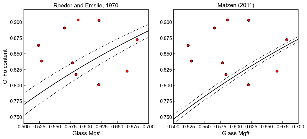
Here, we use these calculated lines, Mg#s and Ol conetnts to draw min and max equilibrium fields for Roeder and Emslie on the LH axis, and Matzen on the RH axis

[26]:

fig, (ax1, ax2) = plt.subplots(1, 2, figsize=(12,5))
# Plotting for Roeder and Emslie
ax1.set_title('Roeder and Emslie, 1970')
# Plotting equilibrium lines
ax1.plot(Rhodes['Mg#_Liq'], Rhodes['Eq_Ol_Fo_Roeder (Kd=0.27)'], ':k')
ax1.plot(Rhodes['Mg#_Liq'], Rhodes['Eq_Ol_Fo_Roeder (Kd=0.33)'], ':k')
ax1.plot(Rhodes['Mg#_Liq'], Rhodes['Eq_Ol_Fo_Roeder (Kd=0.3)'], '-k')

# Plotting data
ax1.plot(Liq_Mgno_calc, Ol_Fo_Calc, 'ok', mfc='red')

ax2.set_title('Matzen (2011)')
# Plotting equilibrium lines
ax2.plot(Rhodes['Mg#_Liq'], Rhodes['Eq_Ol_Fo_Matzen (Kd=0.328)'], ':k')
ax2.plot(Rhodes['Mg#_Liq'], Rhodes['Eq_Ol_Fo_Matzen (Kd=0.352)'], ':k')
ax2.plot(Rhodes['Mg#_Liq'], Rhodes['Eq_Ol_Fo_Matzen (Kd=0.34)'], '-k')
# Plotting data
ax2.plot(Liq_Mgno_calc, Ol_Fo_Calc, 'ok', mfc='red')
ax1.set_ylabel('Ol Fo content')
ax1.set_xlabel('Glass Mg#')
ax2.set_xlabel('Glass Mg#')
# Adjust axis limits here
ax1.set_ylim([0.74, 0.92])
ax2.set_ylim([0.74, 0.92])
ax1.set_xlim([0.5, 0.7])
ax2.set_xlim([0.5, 0.7])

[26]:

(0.5, 0.7)

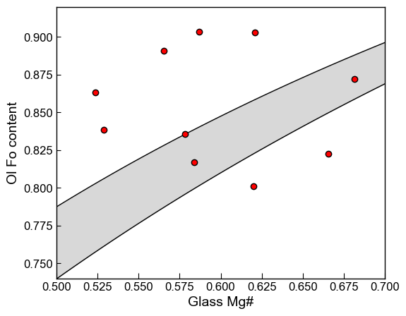
../../_images/Examples_Liquid_Ol_Liq_Themometry_Olivine_Liquid_thermometry_51_1.png

We can also use the fill_between function to show the equilibrium field or you could show the min and max to provide the full range using the fill between function

[27]:

# Calculate Ol Fo contents to plot
Ol_Fo_Calc=pt.calculate_ol_fo(ol_comps=myOls1)
Liq_Mgno_calc=pt.calculate_liq_mgno(liq_comps=myLiquids1, Fe3Fet_Liq=0.2)
## Here we plot these results
fig, (ax1) = plt.subplots(1, 1, figsize=(6,5))

# This section of code fills between the two lines, where xfill_pap is the sorted x co-ordinate,
# and the y1fill and y2fill are the two y coordinates. You have to have a shared x axis (here, same
# generated set of Mg#s)
xfill_pap = np.sort(Rhodes['Mg#_Liq'])
y1fill_pap = Rhodes['Eq_Ol_Fo_Roeder (Kd=0.27)']
y2fill_pap = Rhodes['Eq_Ol_Fo_Matzen (Kd=0.352)']
ax1.fill_between(xfill_pap, y1fill_pap, y2fill_pap, where=y1fill_pap < y2fill_pap,
                 interpolate=True, color='grey',  alpha=0.3)
ax1.fill_between(xfill_pap, y1fill_pap, y2fill_pap, where=y1fill_pap > y2fill_pap,
                 interpolate=True, color='grey', linewidth=0.5, alpha=0.3)


# # Plotting equilibrium lines
ax1.plot(Rhodes['Mg#_Liq'], Rhodes['Eq_Ol_Fo_Roeder (Kd=0.27)'], '-k', linewidth=1)

ax1.plot(Rhodes['Mg#_Liq'], Rhodes['Eq_Ol_Fo_Matzen (Kd=0.352)'], '-k', linewidth=1)
# Plotting data
ax1.plot(Liq_Mgno_calc, Ol_Fo_Calc, 'ok', mfc='red')
ax1.set_ylabel('Ol Fo content')
ax1.set_xlabel('Glass Mg#')
ax1.set_ylim([0.74, 0.92]);
ax1.set_xlim([0.5, 0.7]);

../../_images/Examples_Liquid_Ol_Liq_Themometry_Olivine_Liquid_thermometry_53_0.png

Example 5 - Calculating Fe3Fet_Liq using a buffer position to assess equilibrium

Say we don’t know the Fe3FeT_Liq we want to perform equilibrium calculations at, but we have reason to believe our system is buffered at NNO+1
As liquid-olivine temperatures aren’t sensitive to fo2, first we calculate temperature (as buffers are highly temperature-sensitive)

[28]:

eq22_PHinput=pt.calculate_ol_liq_temp(liq_comps=myLiquids1, ol_comps=myOls1,
                                      equationT="T_Put2008_eq22", P=my_input['P_kbar'])

Then we use this function to convert NNO+1 to a Fe3/FeT ratio (the function returns a dataframe, and the variable we care about is Fe3Fet_Liq)

[29]:

myLiquids_Fe3_Kress_no_norm_Fe3=pt.convert_fo2_to_fe_partition(liq_comps=myLiquids1,
                                T_K=eq22_PHinput['T_K_calc'], P_kbar=3, fo2="NNO", fo2_offset=1,
                                model="Kress1991", renorm=False).Fe3Fet_Liq
myLiquids_Fe3_Kress_no_norm_Fe3

[29]:

0    0.286549
1    0.294522
2    0.290725
3    0.304642
4    0.288451
5    0.293145
6    0.296381
7    0.276202
8    0.290563
9    0.278905
Name: Fe3Fet_Liq, dtype: float64

We then input this into the calculate_ol_liq_temp function as Fe3Fet_Liq=….

[30]:

eq22_PHinput_EqTests=pt.calculate_ol_liq_temp(liq_comps=myLiquids1, ol_comps=myOls1,
                                      equationT="T_Put2008_eq22", P=my_input['P_kbar'], eq_tests=True,
                                    Fe3Fet_Liq=myLiquids_Fe3_Kress_no_norm_Fe3)
eq22_PHinput_EqTests

[30]:

	T_K_calc	Kd Meas	Kd calc (Toplis)	ΔKd, Toplis (M-P)	ΔKd, Roeder (M-P)	ΔKd, Matzen (M-P)	SiO2_Liq	TiO2_Liq	Al2O3_Liq	FeOt_Liq	...	Sample_ID_Ol	Fo_meas	DMg_Meas	CNML	CSiO2L	NF	Den_Beat93
0	1289.947705	0.352387	0.325040	0.027347	0.052387	0.012387	57.023602	0.623106	16.332899	4.36174	...	0	0.872023	9.472619	0.170395	0.557471	-0.761843	9.819071
1	1229.813416	0.198881	0.308684	-0.109802	-0.101119	-0.141119	57.658600	0.654150	17.194799	3.90621	...	1	0.903203	14.186789	0.137941	0.570023	-0.816654	10.303635
2	1285.857491	0.304065	0.315891	-0.011826	0.004065	-0.035935	60.731201	0.862054	17.144199	4.07781	...	2	0.835656	15.531216	0.122184	0.579288	-0.792785	10.250501
3	1198.240159	0.199954	0.296719	-0.096765	-0.100046	-0.140046	61.532799	0.440860	16.508801	3.32990	...	3	0.863386	23.753206	0.097626	0.605753	-0.767076	10.715090
4	1259.174284	0.171088	0.323766	-0.152678	-0.128912	-0.168912	52.969101	0.803412	17.563000	5.93217	...	4	0.903278	10.781292	0.186877	0.523030	-0.842157	10.215321
5	1244.931462	0.180579	0.324986	-0.144407	-0.119421	-0.159421	54.050201	0.857348	17.333300	5.60072	...	5	0.890781	12.276130	0.168070	0.533835	-0.833465	10.295063
6	1241.300118	0.245491	0.333878	-0.088387	-0.054509	-0.094509	55.656300	0.897984	17.117800	5.31307	...	6	0.838609	14.083460	0.145845	0.547483	-0.820914	10.324021
7	1199.601831	0.447306	0.391378	0.055928	0.147306	0.107306	49.054699	0.488832	14.665000	5.83168	...	7	0.801278	7.372298	0.220053	0.554209	-0.789502	9.845140
8	1162.693468	0.354214	0.361834	-0.007620	0.054214	0.014214	50.625099	0.334074	16.875000	5.01968	...	8	0.817074	10.509878	0.180293	0.551305	-0.873502	10.229233
9	1339.466029	0.476093	0.299720	0.176373	0.176093	0.136093	51.403301	0.663880	18.019600	5.98440	...	9	0.822724	7.070601	0.228386	0.498172	-0.840523	9.673734

10 rows × 75 columns

[ ]:

[ ]:

[ ]: